How To: Create a Three-Step Kinetic Model for Dilatometer (DIL) Data

Sintering of Si₃N₄

Introduction

During the sintering process the shrinkage of the testing material could be observed. Length change of the sample can be measured by dilatometers.

In this How To: guide, a three-step kinetic model will be created for dilatometer measurement of sintering process.

We will start by loading a sample data project included in Kinetics Neo, will then create a three-step model and finally will optimize it.

Sample data:

Data Type: Dilatometry (DIL)
Project File: Si3n4_I_Data.kinx2

Load the Sample Data Project

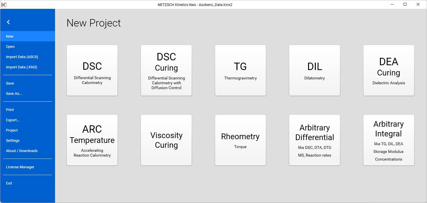
1. Start the Kinetics Neo software.

Click on the File tab on the main top ribbon to open the application menu.

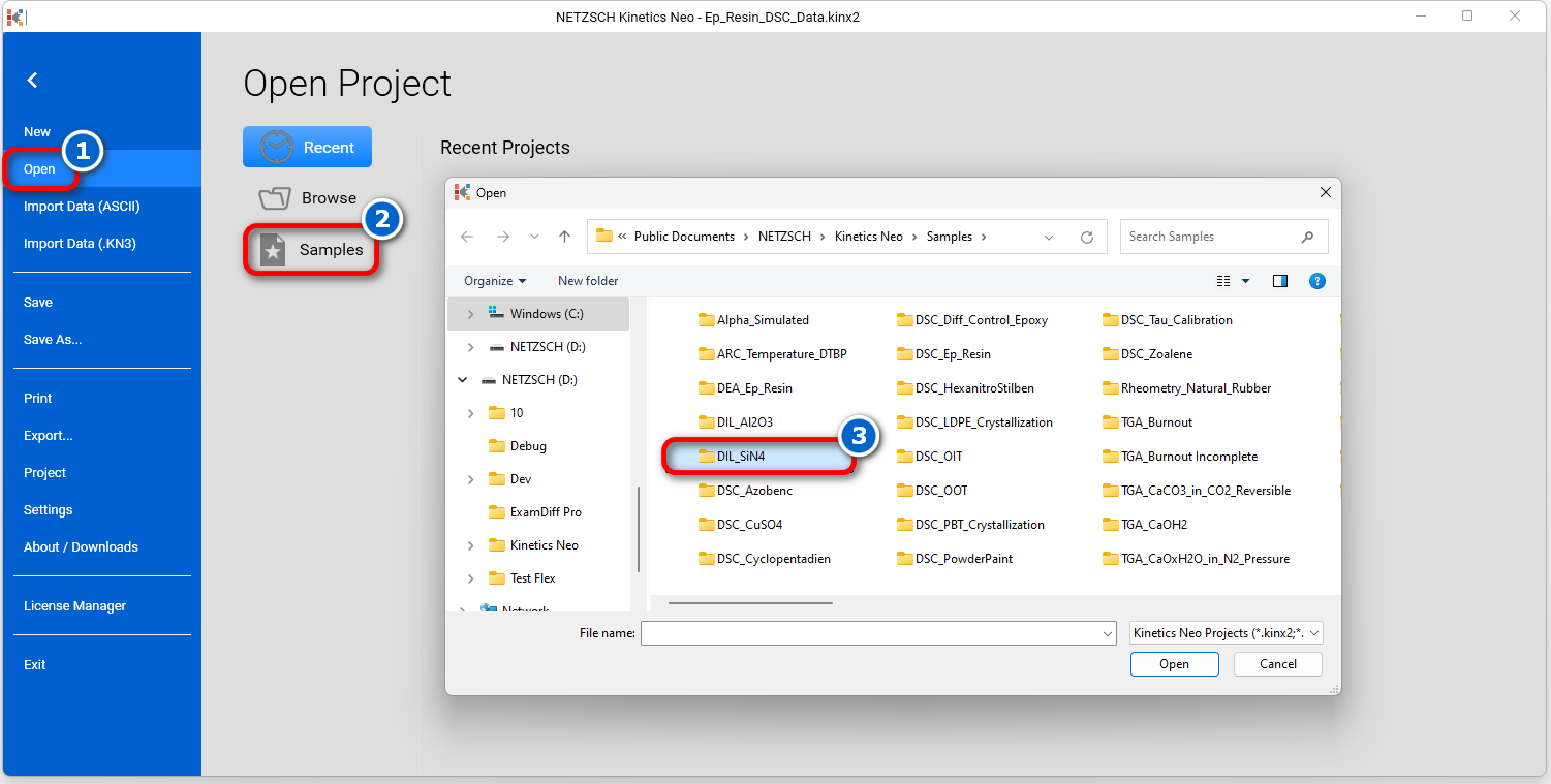
2. Open the Sample Data DIL project.

Click on Open in the panel on the left panel, then select Samples. The Kinetics Neo samples directory will open in Windows Explorer. Select the DIL_Si3N4 directory.

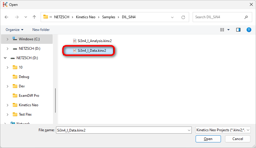
3. Open the Kinetics Neo project file Si3n4_I_Data.kinx2.

Check the Loaded Measurement Data

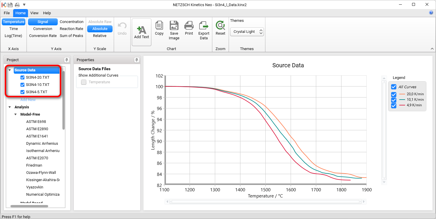
4. Check whether the DIL measurement data are loaded.

The Kinetics Neo sample project Si3n4_I_Data.kinx2 already contains imported dilatometer measurement data files for the sintering of Si3N4:

Si3N4-20.txt - heating rate 20 K/min
Si3N4-10.txt - heating rate 10 K/min
Si3N4-5.txt - heating rate 5 K/min.

If the project file is successfully loaded, then these file names will be seen in the “Source Data” section on the left side. The data curves will be shown on the main chart.

After - Import Sample Data Preparation

By clicking on one of the sample data files it would be possible to narrow the temperature range by selecting a left and a right cursor position. In addition smoothing of the data can be done if necessary.

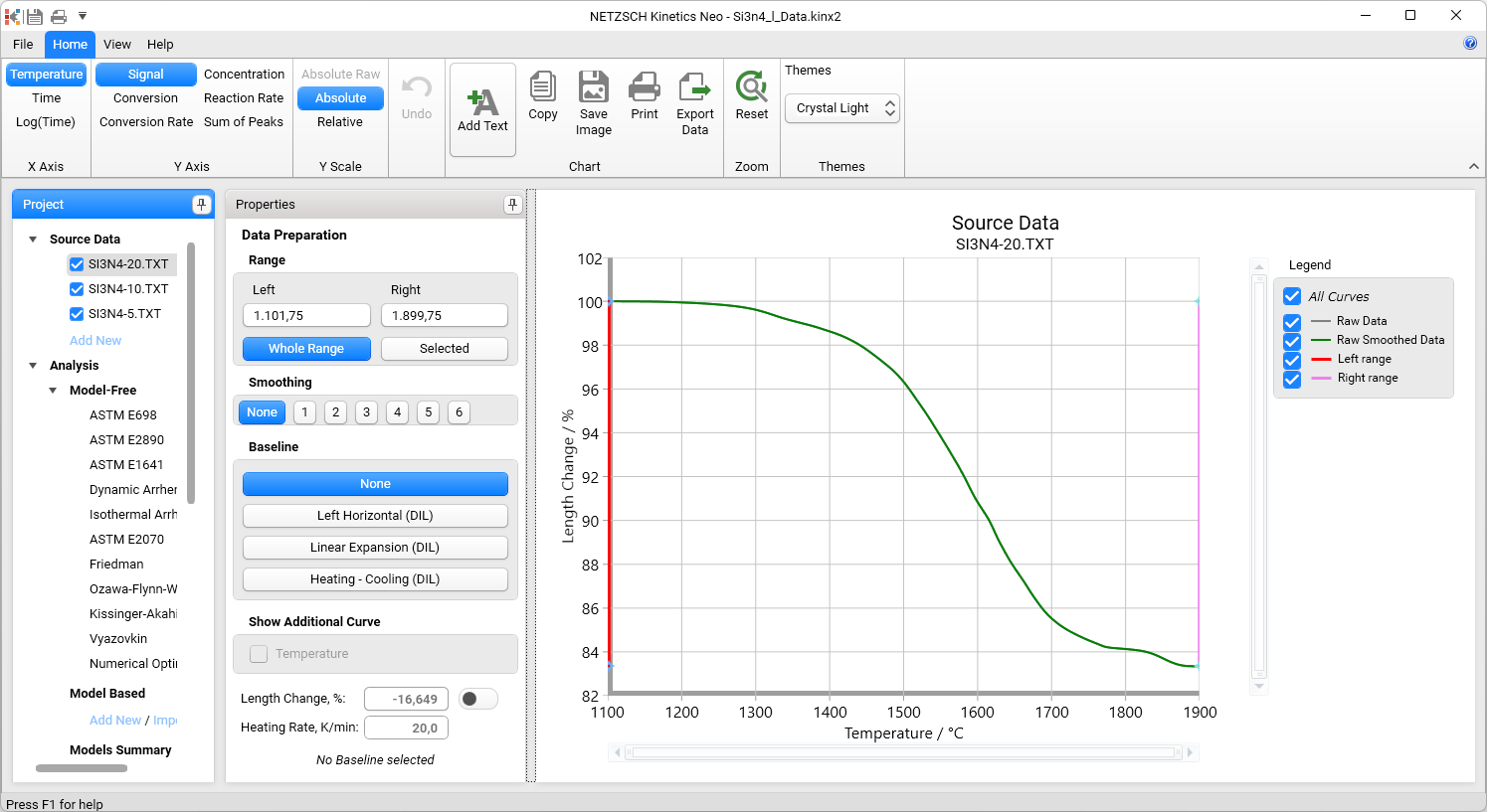
For sintering processes an assumption can be made about the expansion of the material without sintering. Therefore a baseline can be selected. The options are:

None
Left Horizontal (DIL)
Linear Expansion (DIL)
Heating – Cooling (DIL) - It is only possible if cooling data is contained in the measurement file.

For this “How To:”, no baseline was selected because the data contain no thermal expansion.

Create a One-Step Kinetic Model

5. In the left Analysis panel, under Model Based, item click on Add New.

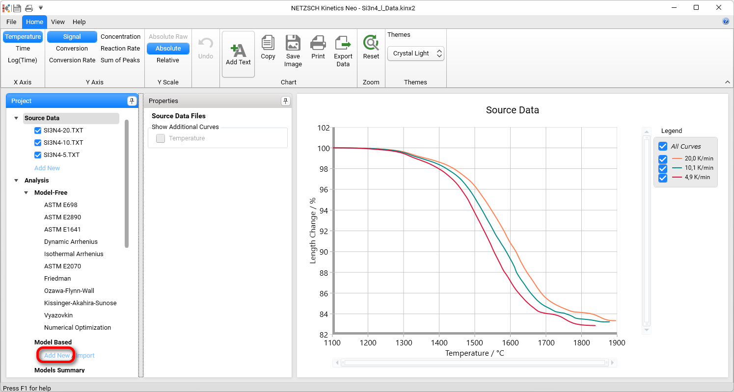
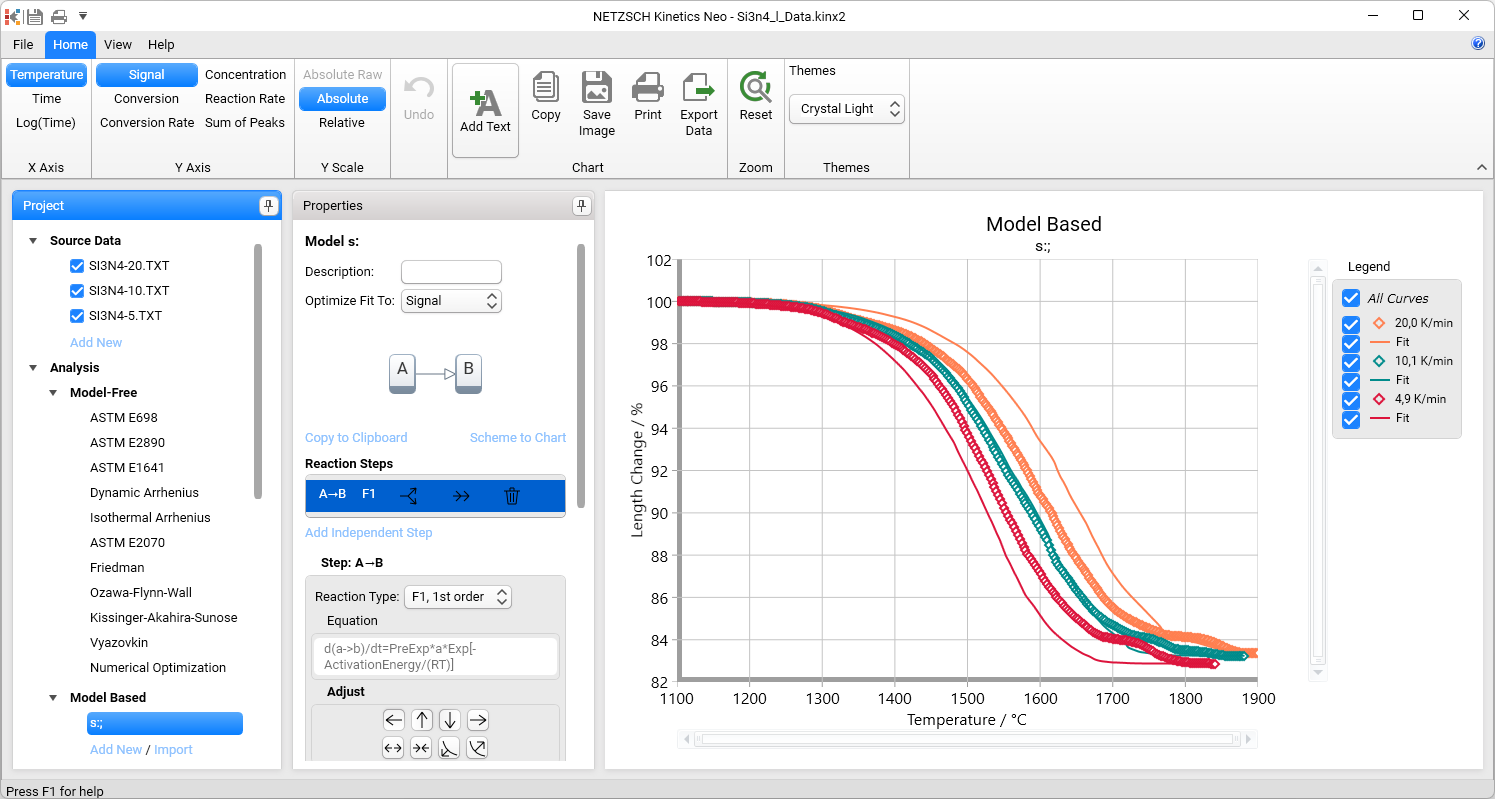
A new Model Based kinetic model will be created.

This new model has the following default parameters:

One step: A → B
Reaction Type: F1, 1st order.

Sintering processes are quite complex as several reactions take place, sometimes simultaneously. Therefore we cannot be sure that this and the following reactions have the reaction order 1. In this case, it is recommended to select the general reaction order n, which would also include the value of 1. Using model optimization, the software will determine the correct reaction order on its own.

First of all, in the Reaction Type drop-down menu, change the reaction type from the default value F1, 1st order to Fn, n-th order. Then, within Model Operations, click on the Optimize button.

IMPORTANT: do model optimization BEFORE you insert additional steps.

It should be the first action after model creation and defining the reaction type.

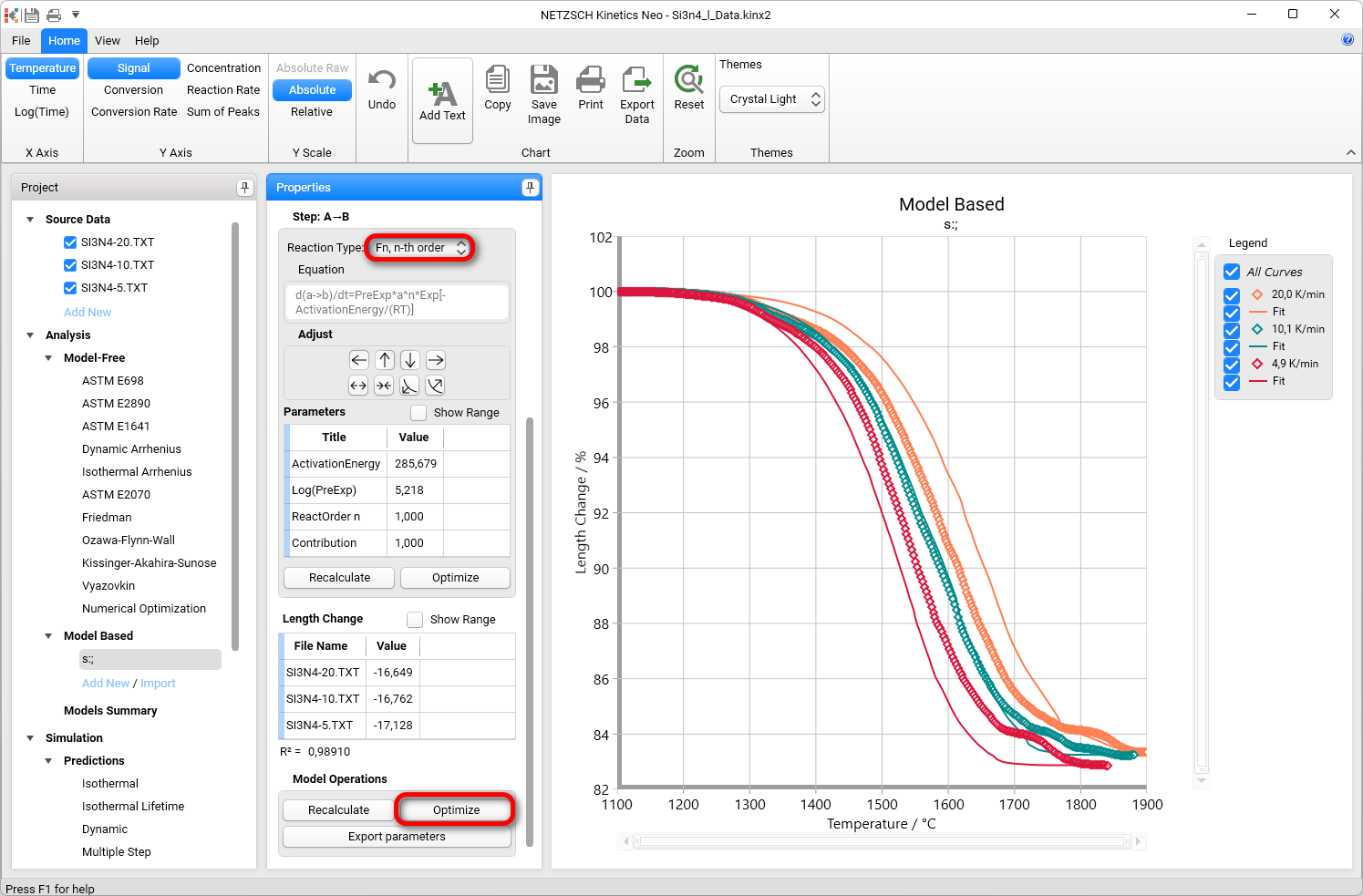
After model optimization all model parameters are recalculated to fit the source data.

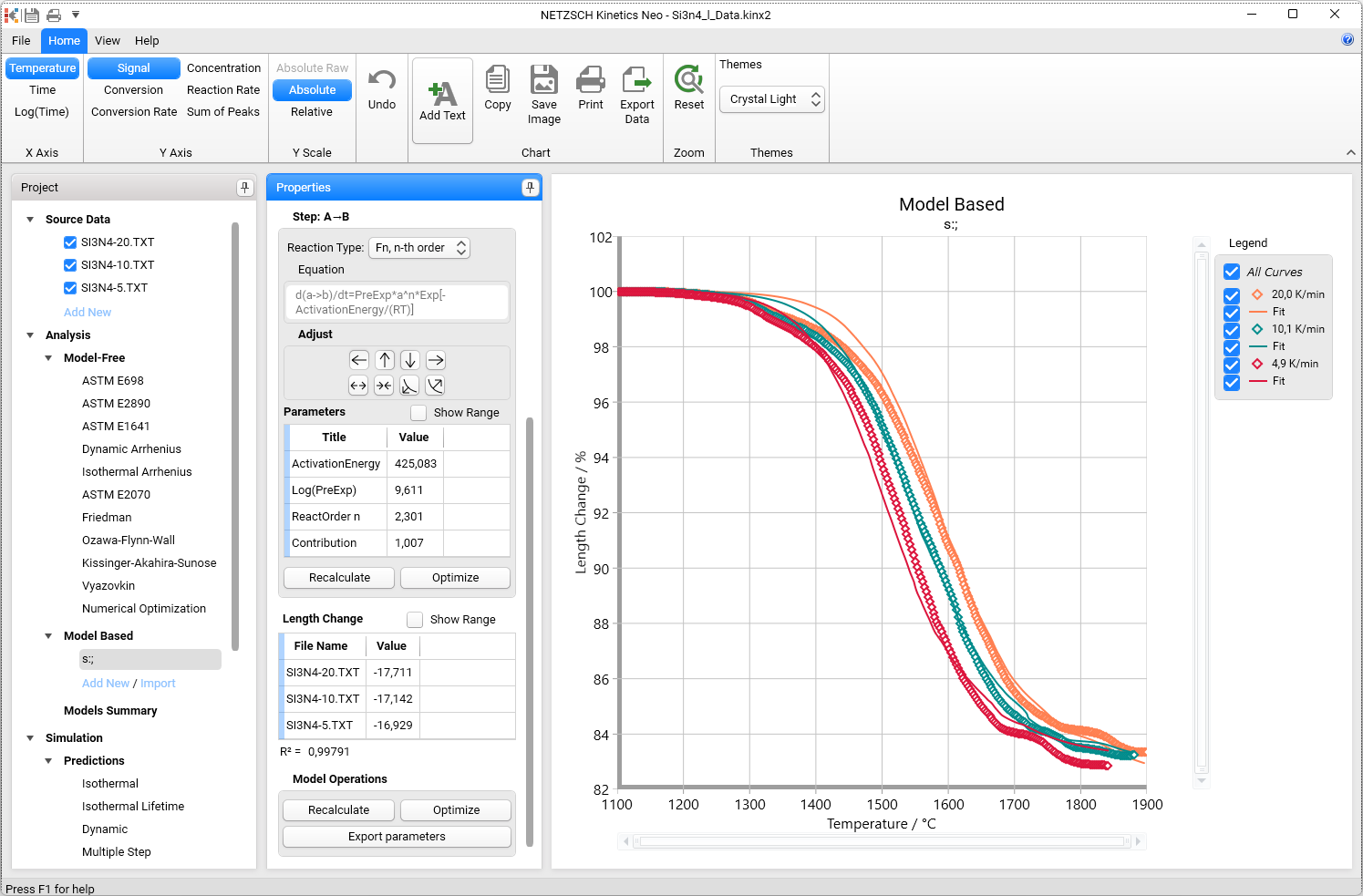
This simulated curves for this one-step model have not the good agreement with the experiment. Therefore the second reaction step is necessary.

Why and Where to Add the New Kinetic Steps?

6. Please switch to Conversion Rate in the top ribbon panel.

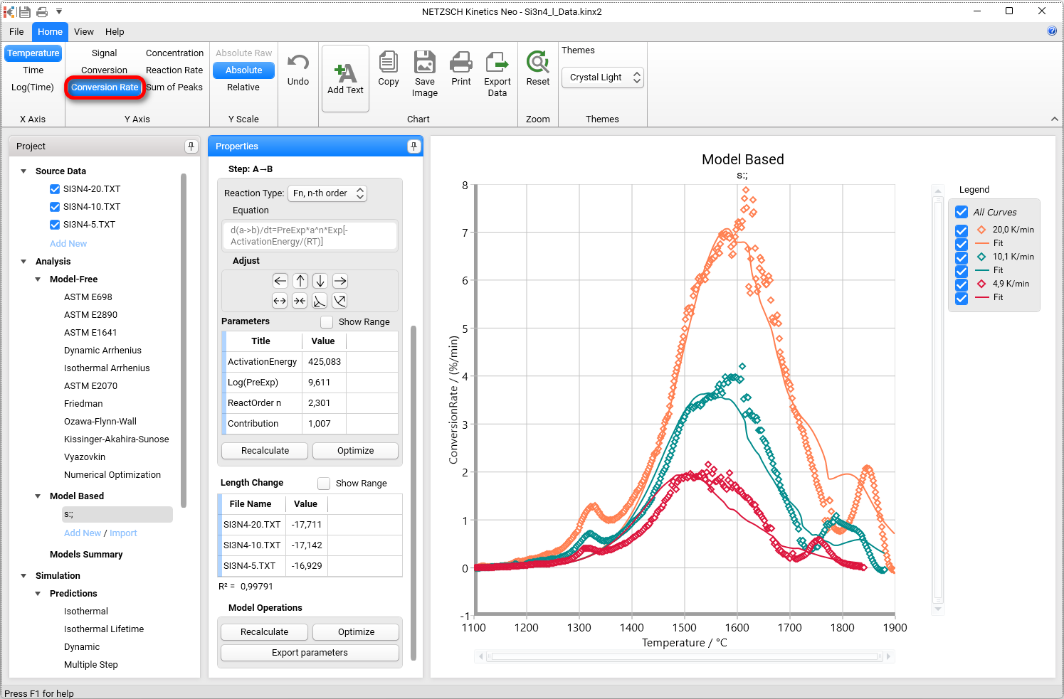
Here we have fit only for the main peak at 1600 °C. The first small peak at 1320 °C is seen on the raw data but is not present in the simulated curves. The main peak looks as the double peak. For example, the green measurement 10 K/min has the double peak with maxima at 1500 °C and 1600 °C. The last experimental peak at 1800 °C has a corresponding peak in the simulated curve. Therefore it comes probably from the nonlinearity of the temperature and probably does not require the reaction step in the model.

Firstly we will add the small peak at 1320 °C. After that we will expand the main peak to the double peak.

Let us add the first peak. This small peak is finished at approximately 1370 °C. Let us find its contribution.

Switch to Conversion on the top ribbon panel.

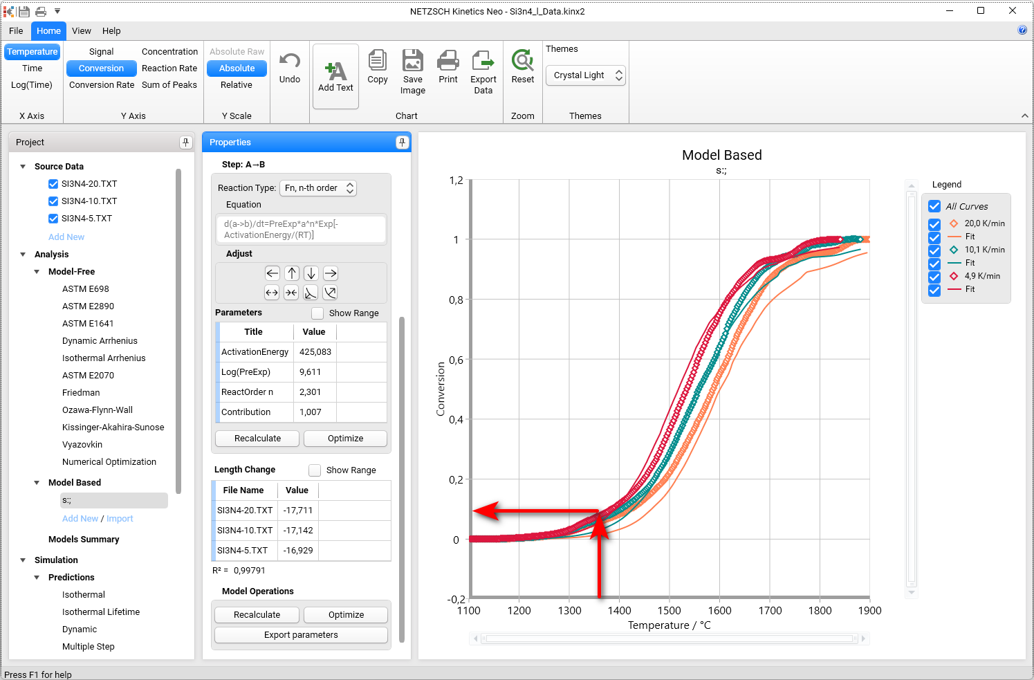
The experimental curves have at 1370 °C the conversion value about 0.08. This is the contribution of our first reaction step. Then the second step must have the contribution 0.92 in order to have 1.0 in the sum.

Now we will add the new reaction step with contribution 0.08 before the main step.

Create a Kinetics Model with Two Consecutive Steps

7. A new Model Based kinetic model with two consecutive steps will be created.

Switch to the Signal on the top ribbon panel.

We will use the existing model and duplicate it. To do this, in left Project panel under Model Based, make a right-mouse-click over our model s; and in context menu select + Copy.

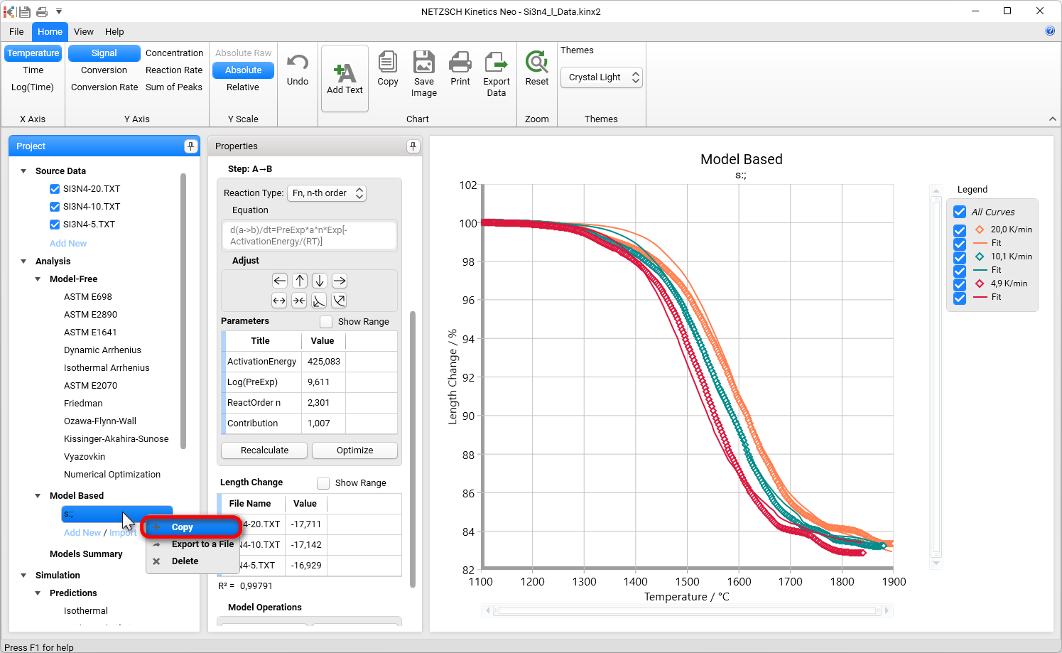
A new model, copied from the first model, will be created.

8. Within the Reaction Step: A → B, create a consecutive step by clicking on →→ .

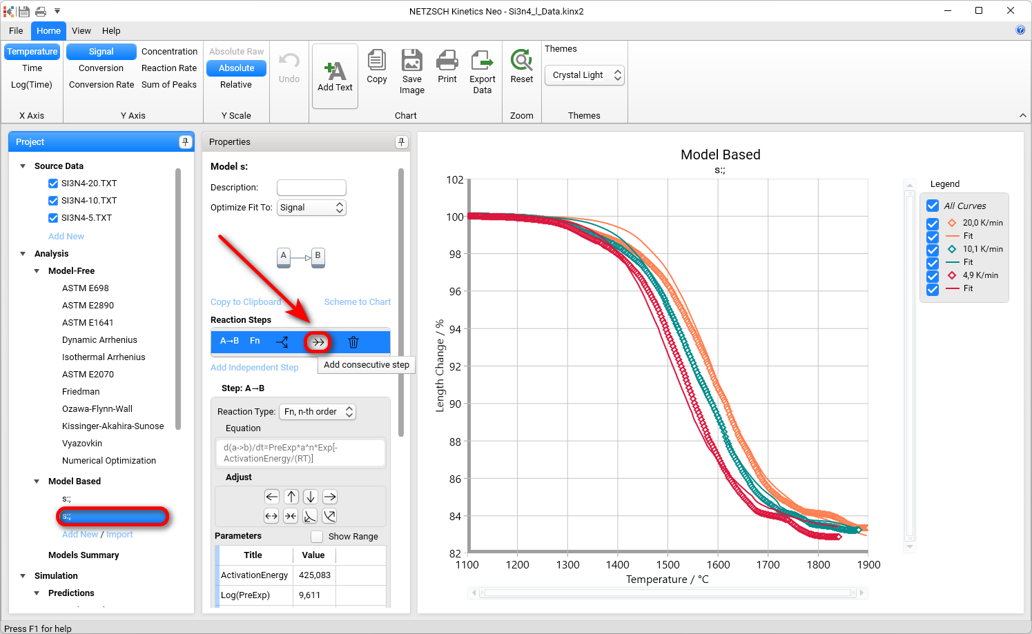
A two-step model will be created.

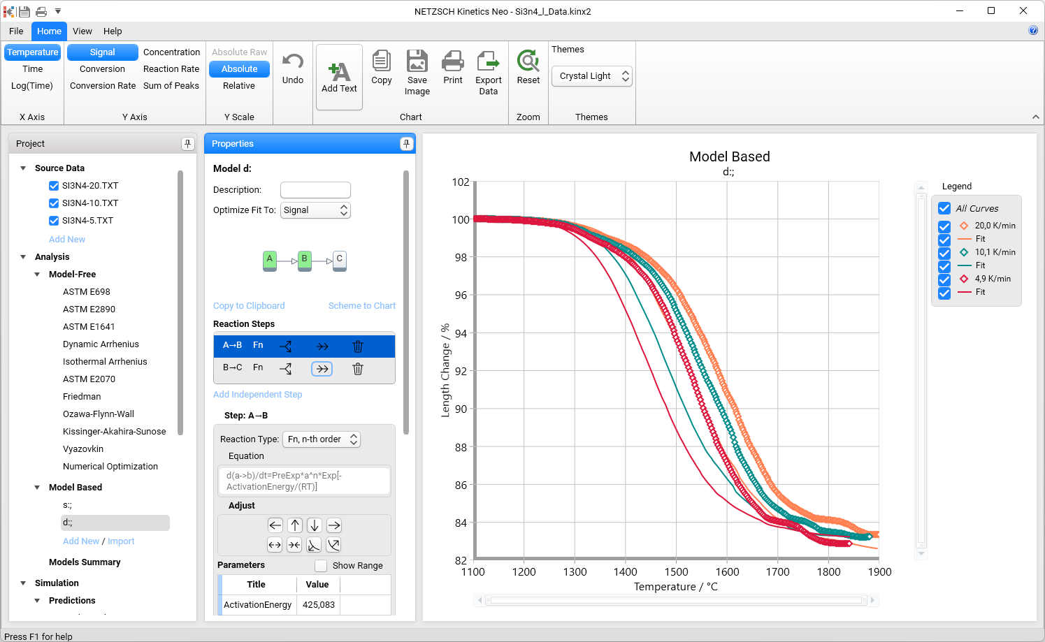
9. Select the first step A → B and set its contribution 0.08.

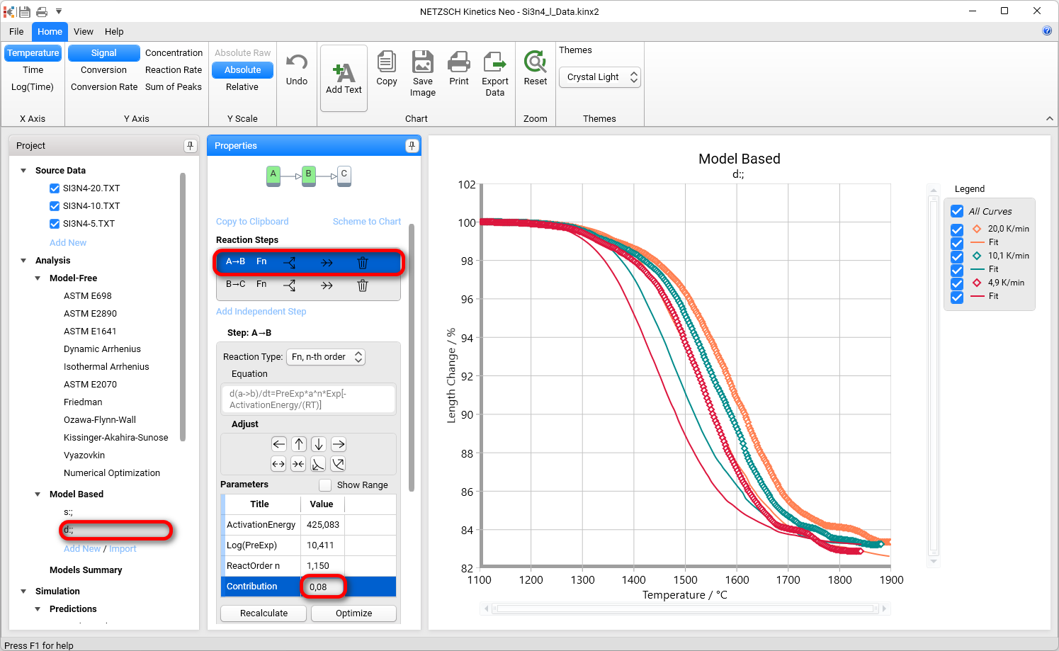
10. Select the second step and set its contribution to 0.92.

In Step B → C region click on Recalculate button.

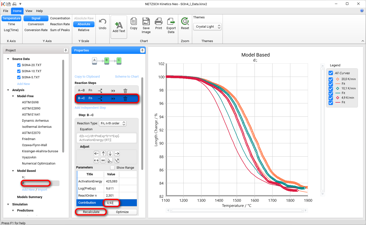
11. Now the simulated data for the initial part of the model are placed right to experimental data. Select the first step A → B and move it to the left by pressing the Adjust button: "←".

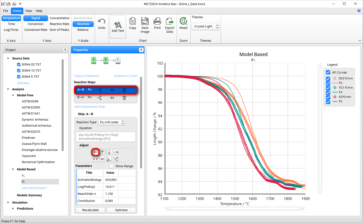
Now the simulated curves are not far from the experimental data, and we can do the optimization.

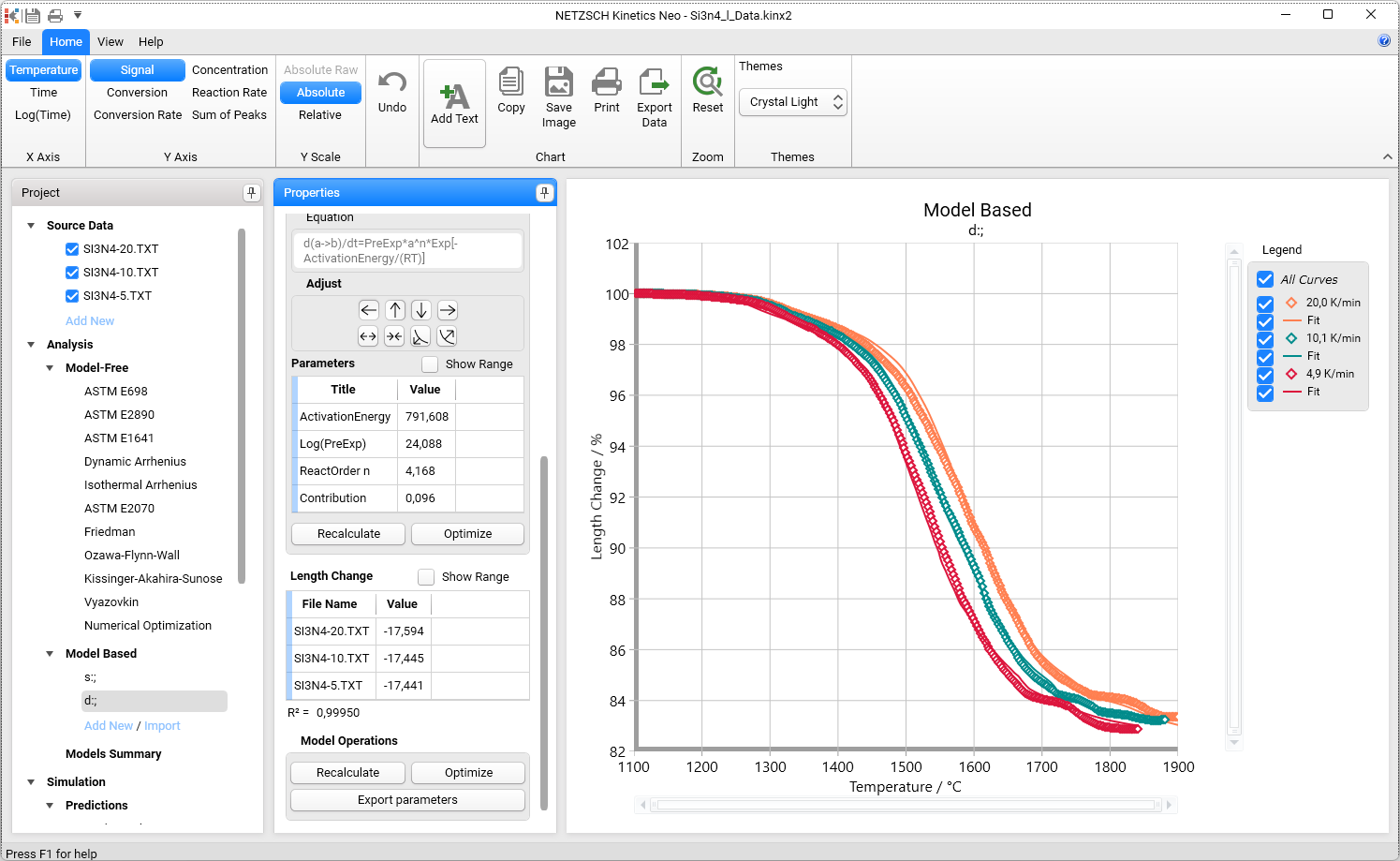
In Model Operations click on button Optimize.

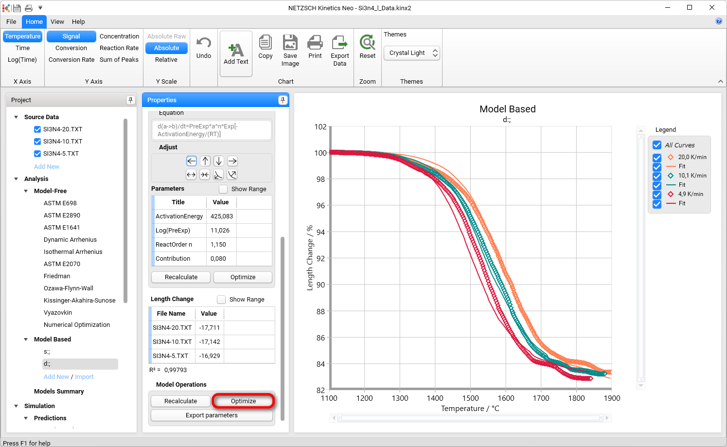
Now the double-step model is ready.

Create a Kinetics Model with Three Consecutive Steps

12. A new Model Based kinetic model with three consecutive steps will be created.

We will use our second, double-step model d; and duplicate it. To do this, under Model Based, select double-step model, make a right-mouse-click on it and in context menu select + Copy. An existing model d; will be copied and a new model will be created.

Select this new model. Here we will add a new, third reaction step.

Please select step (B →C) and add consecutive step by clicking on →→. Afterward, under Model Operations click on Optimize to optimize the whole kinetic model.

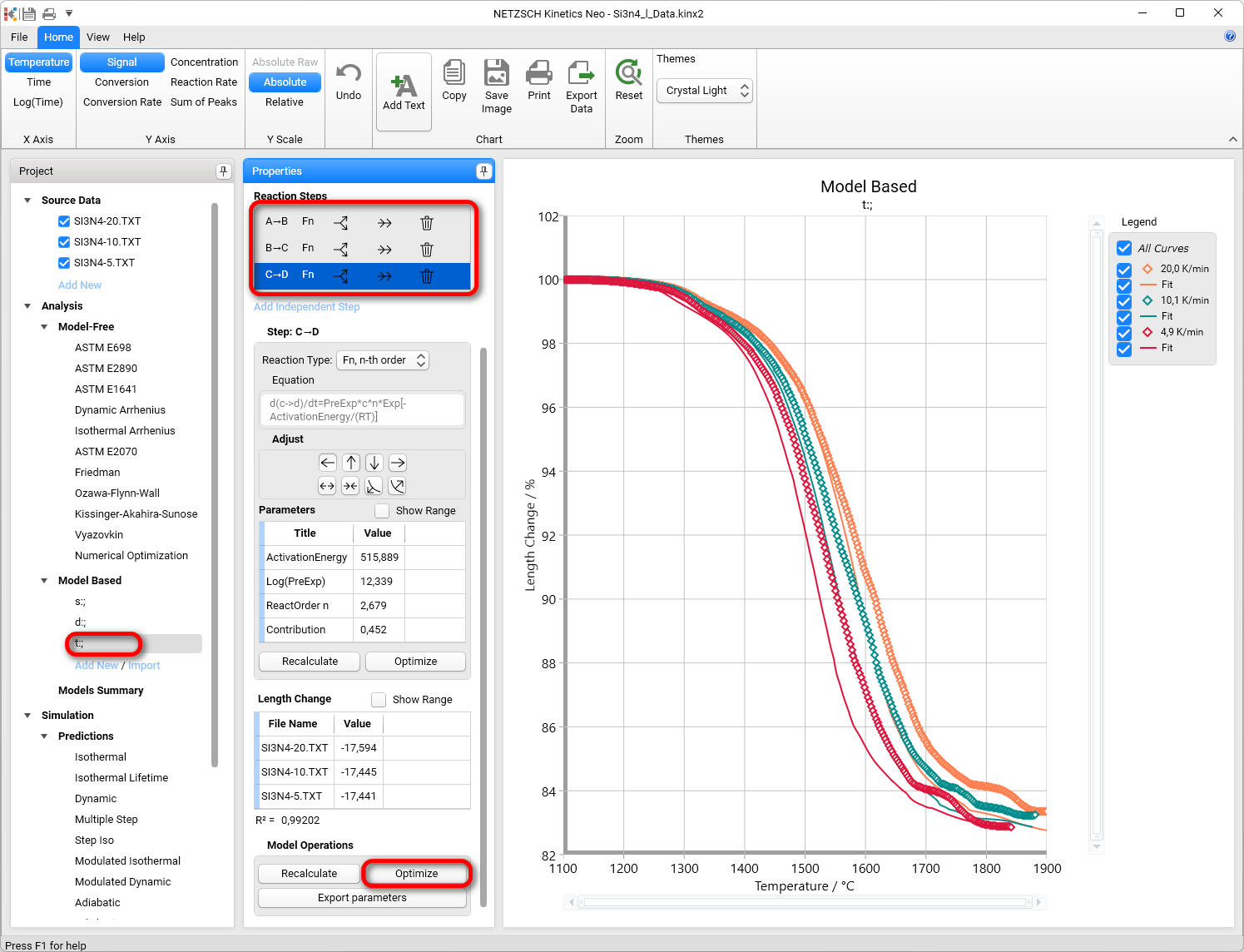
Now the three-step model is ready:

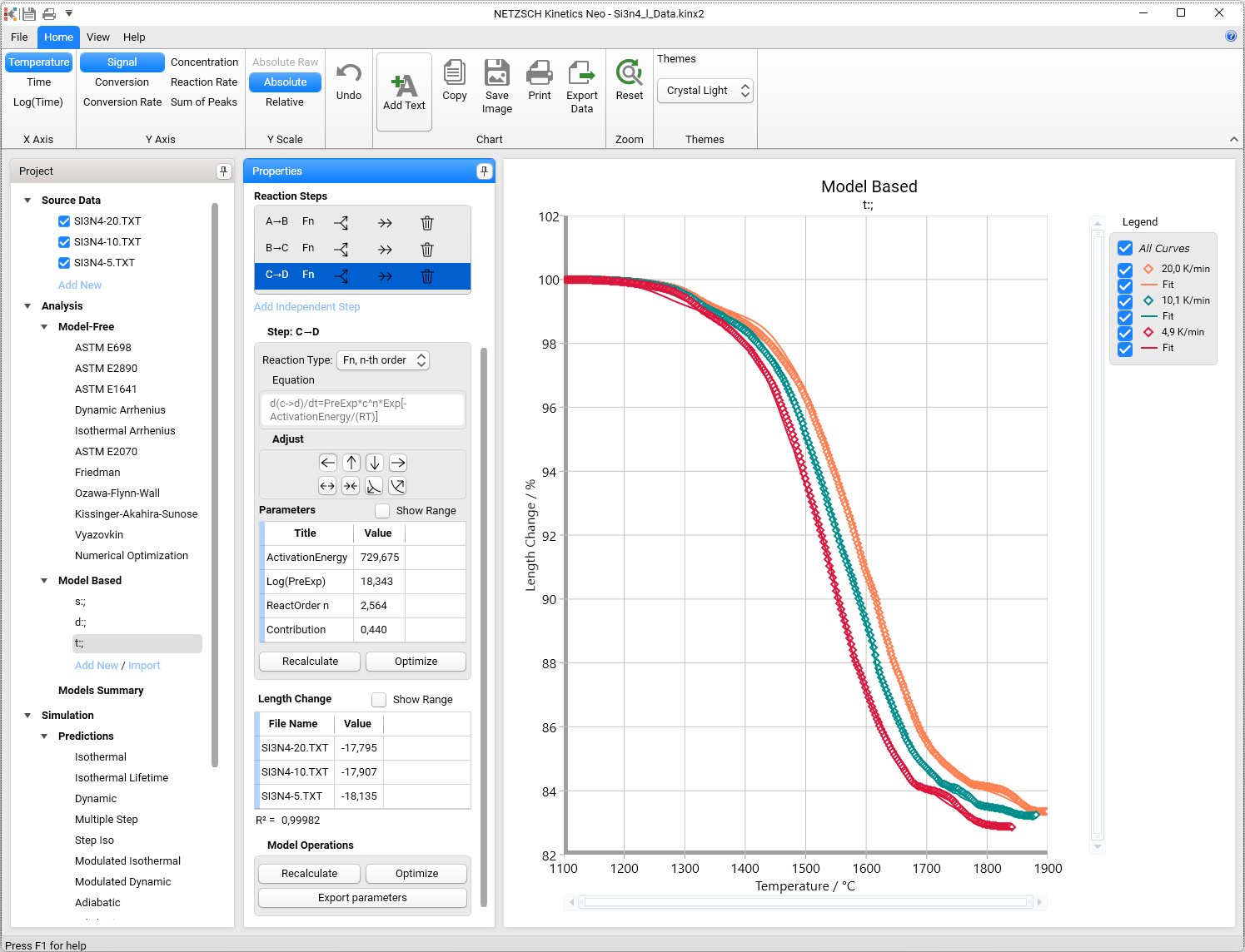
Model Summary

13. By clicking on Models Summary on the left panel, you can see a comparison of some statistical parameters such as the correlation coefficient, R², or the F-Test for the three models that were created during this How To: guide.

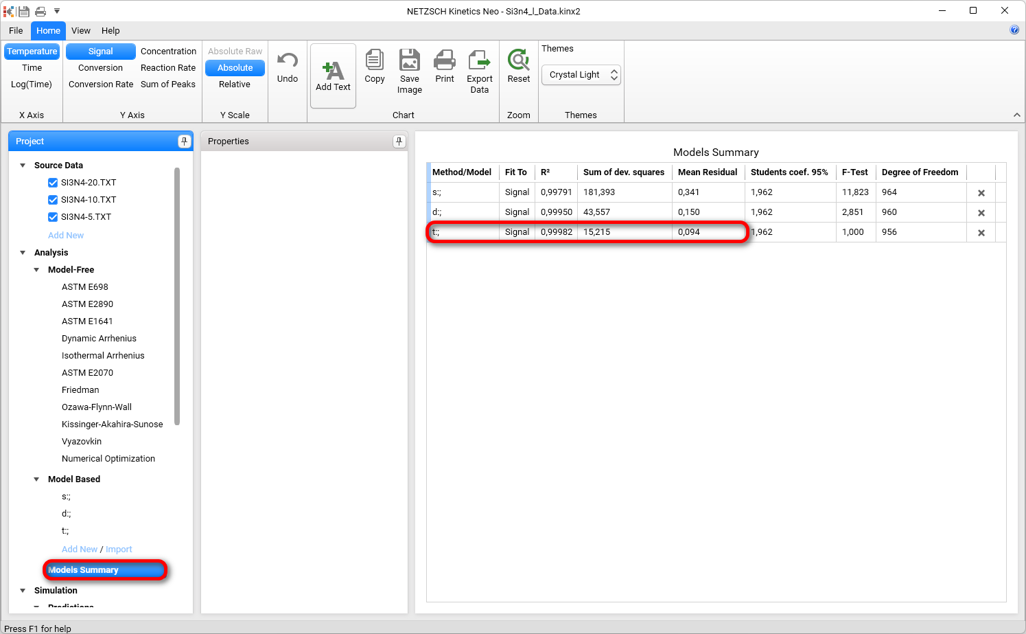
The three-step model is much better because it has a higher R², a lower F-Test, lower sum of deviation squares and a lower mean residual.