How To: Create a Simple Single Step Kinetic Model for DSC Data

Load the Sample Data Project

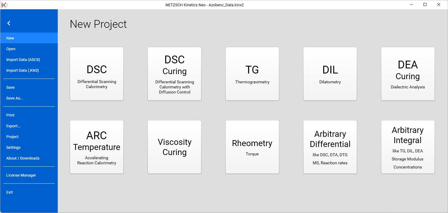
1. Start the Kinetics Neo software.

Click on the File tab to open the top application ribbon.

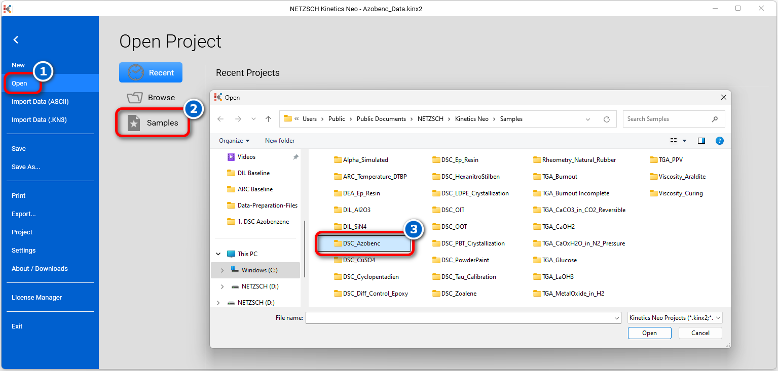
2. Open the Sample Data DSC project.

Click on Open in the menu on the left side, then select Samples. The Kinetics Neo samples directory will be opened in Windows Explorer. Select the directory DSC_Azobenc.

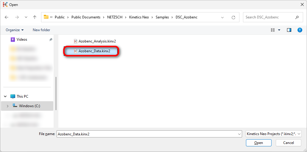
3. Open the Kinetics Neo project file Azobenc_Data.kinx2.

Check the Loaded Measurement Data

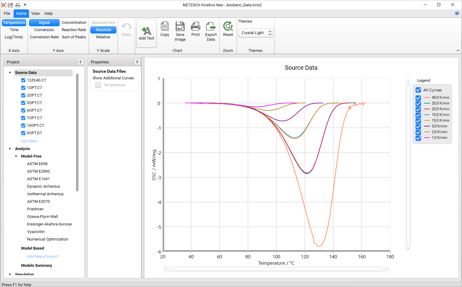
4. Check whether the DSC measurement data are loaded.

The Kinetics Neo sample project Azobenc_Data.kinx2 already contains imported sample DSC measurement data files for sample isomerization:

• 12ZK40.C7- heating rate 40 K/min
• 1OPT.C7 - heating rate 20 K/min
• 2OPT.C7- heating rate 20 K/min
• 5OPT.C7- heating rate 10 K/min
• 6OPT.C7- heating rate 10 K/min
• 7OPT.C7- heating rate 5 K/min
• 1OOpt.C7- heating rate 2 K/min
• 9OPT.D7- heating rate 1 K/min.

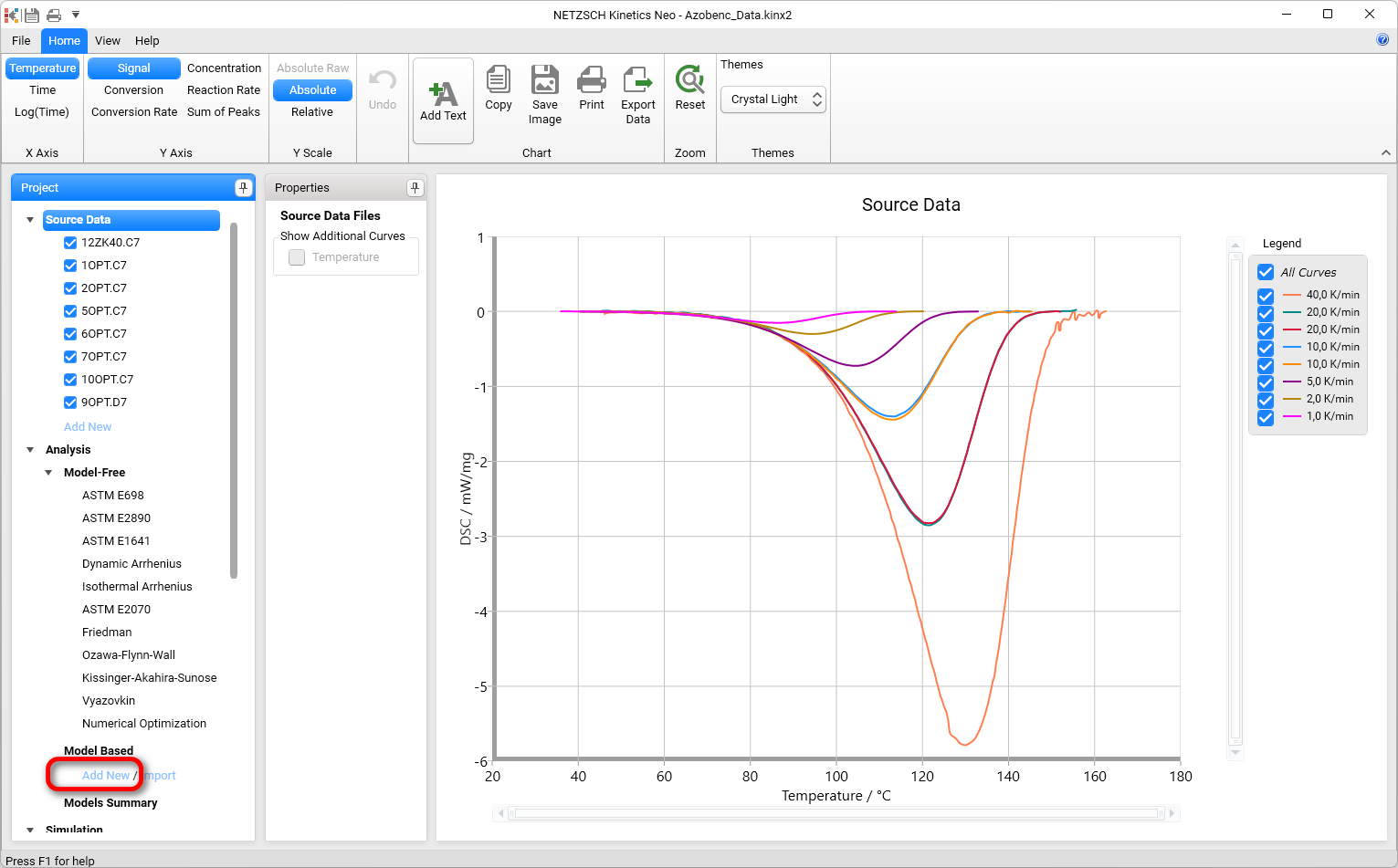
If the project file is successfully loaded then these file names will be seen in the Source Data section on the left panel. The data curves will be shown on the main chart.

Create a One-Step Kinetic Model (F1)

5. Add new model: In the left Analysis panel under Model Based click on Add New.

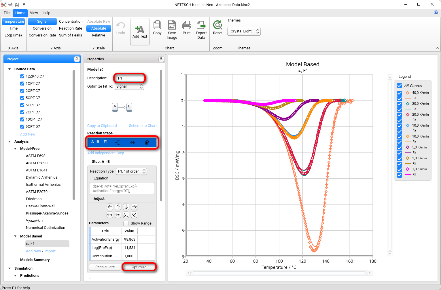
A new Model Based kinetic model will be created with default parameters:

• One step: A → B
• Reaction type: F1, 1st order reaction.

The first model step A → B will be selected.

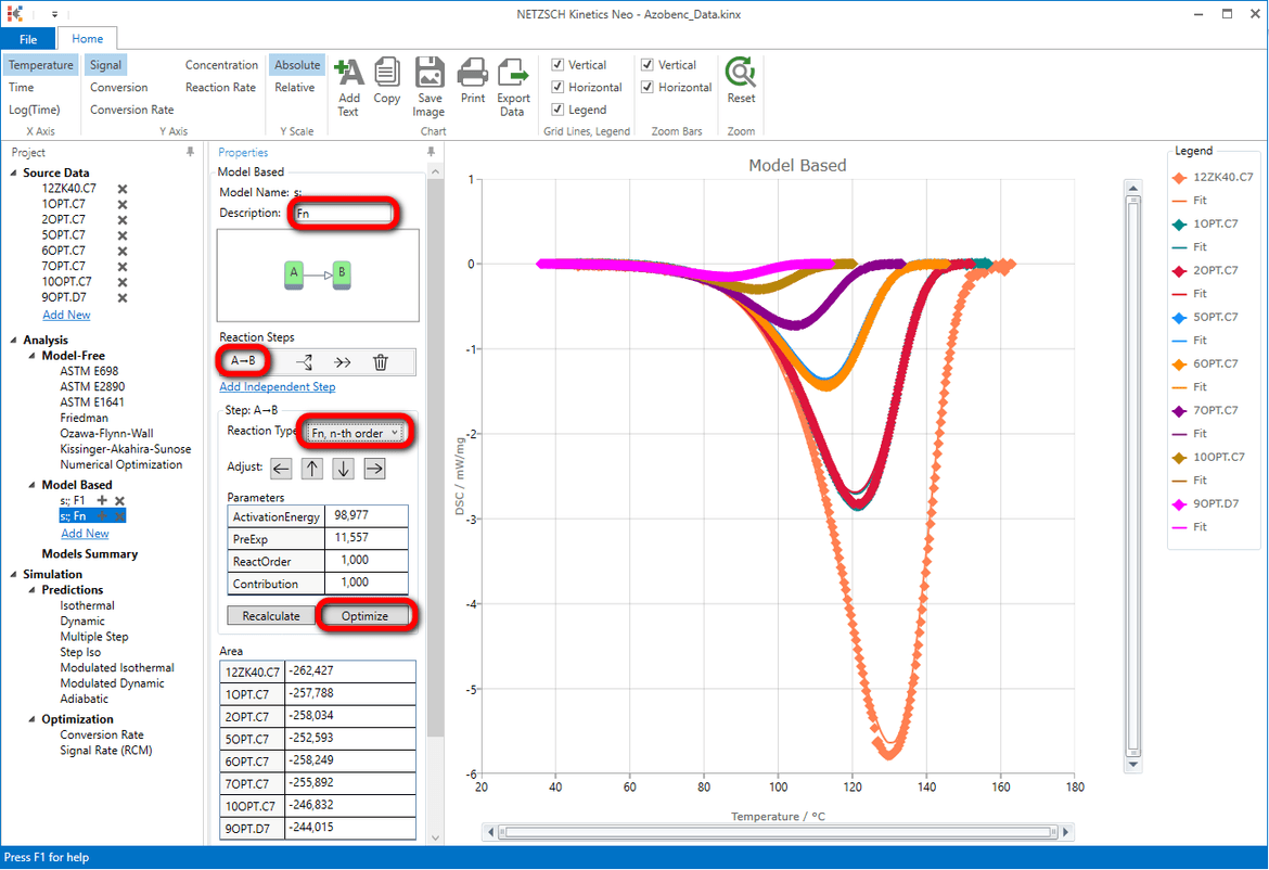
Optionally you can type F1 into the model description text box.

Then, within the step: A → B section, click on Optimize button. The model step parameters: activation energy, pre-exponential factor and contribution will be recalculated and optimized for the this step.

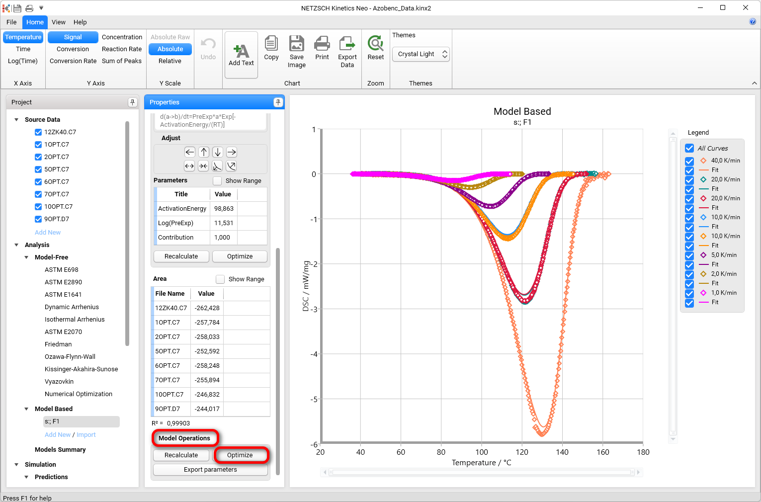
6. Optimize one-step model F1.

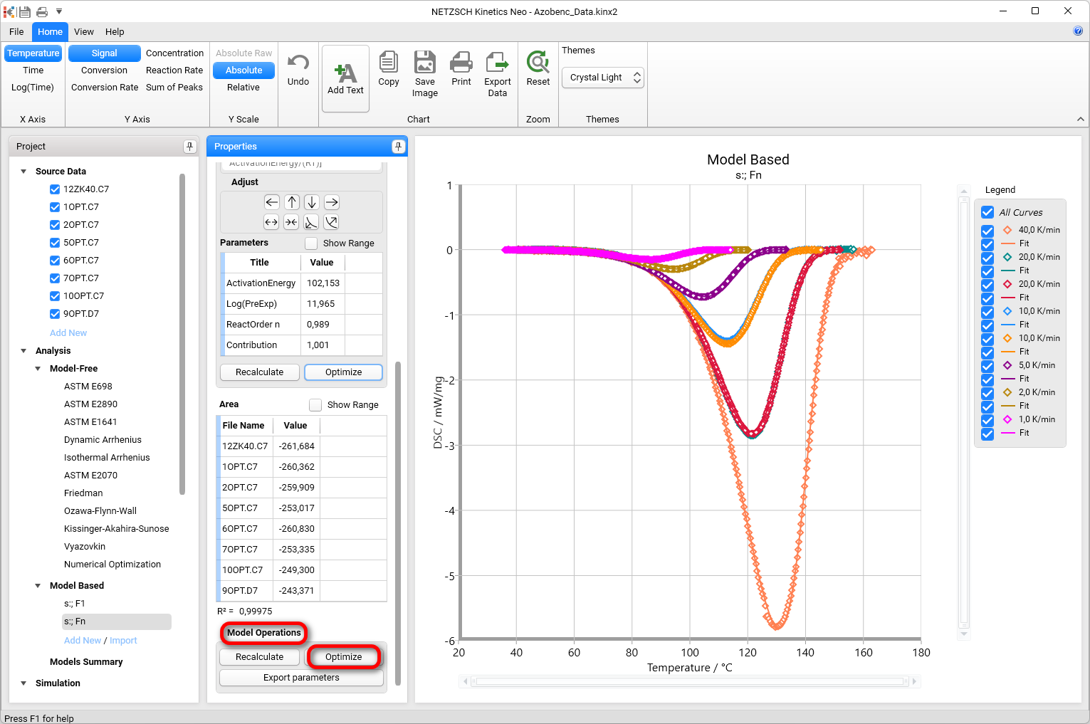
In Model Operations section at the lower part of Properties panel select Optimize. The whole model will be optimized. This may take a few seconds...

Result after model optimization:

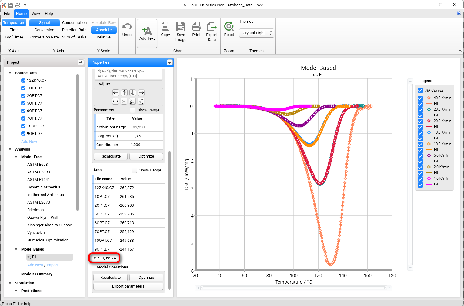
The coefficient of correlation is quite high: R=0.99974 .

Is it good enough?

It is possible to try another model with, for example, a different reaction type and compare the model results with each other. As an example, one may attempt to get a better adaptation of the calculated curves to the measured curves with a reaction type of Fn (n-th order reaction). Then one can assess whether it better fits the source data.

Create a Second One-Step Kinetic Model (Fn). Optional

7. Add new model: In the left Analysis panel under Model Based click on Add New.

A new Model Based kinetic model will be created with the default parameters:

• One step: A → B
• Reaction type: F1, 1st order reaction.

First reaction step A → B with reaction type F1 will be selected.

In order to distinguish two models type a Fn into the Description text box. in Reaction Type dropbox change the default reaction type F1 to Fn, n-th order. Then, within the Step: A → B section, click on Optimize button. The model step parameters: activation energy, pre-exponential factor and contribution will be recalculated and optimized for the this step.

8. Optimize the one-step model Fn.

In the Model Operations section in the lower part of the Properties panel select Optimize. The whole model will be optimized. This may take a few seconds...

Result after model optimization:

Compare the Two Models. Optional

You can compare the statistics of the different calculated models by clicking on Model Summary in the left Analysis panel.

A closer look on the coefficients of correlation of both models F1 and Fn shows that they are nearly the same.

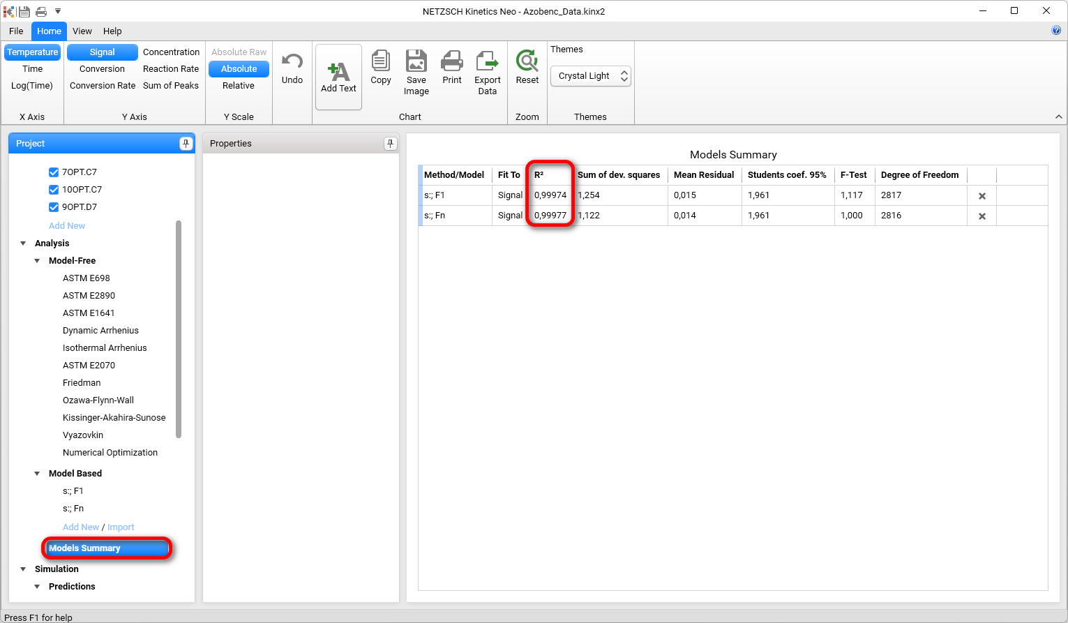
Now we have two models. One is s:; F1 contains one reaction step F1 with the first order reaction. The second is s:; Fn contains also one reaction step, but with reaction of n-th order. The value n is more general and can have any numeric value including one.

It is interesting to check which value has the reaction order in the second model.

In Analysis left panel under Model Based select the second model s:; Fn. 

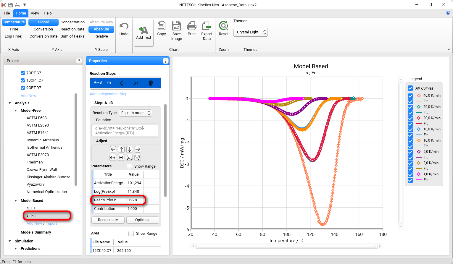
Conclusion

The reaction order of the model s:; Fn is nearly 1 (0.978). The model F1 is in fact the model Fn with fixed  reaction order 1. This explain why the results of the models F1 and Fn are very similar.

This corresponds to the literature values of the first order reaction for Cis-trans isomerization of subcooled liquid Azobenzene from the following article:

Eckardt, N., Flammersheim, H.J. & Cammenga, H.K. The cis-trans Isomerization of Azobenzene in the Molten State: A useful test reaction for the kinetic evaluation of DSC measurements. Journal of Thermal Analysis and Calorimetry  52, 177–185 (1998), https://doi.org/10.1023/A:1010178610642