How To: Create a Single Step Kinetic Model for DEA Data

Introduction

In this How To:  guide a single step kinetic model for DEA data will be created.

We will start with loading of sample data project included in Kinetics Neo, and create a kinetics model consists of one main step.

Only several clicks in several minutes - and you will get your kinetics model!

Sample Data

• Data type: Dielectric Analysis (DEA)
• Project file: DEA_Ep_Resin_Data.kinx2 .

Load the Sample Data Project

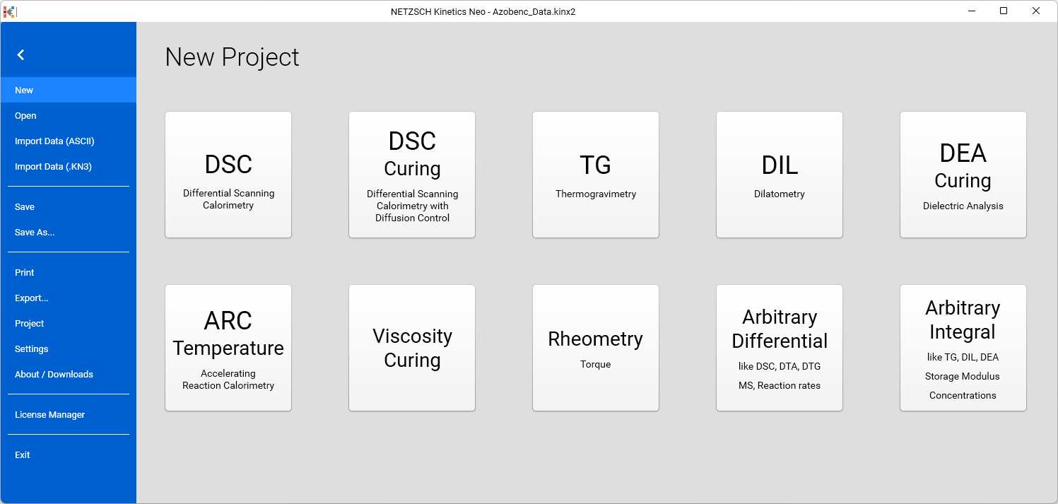
1. Start Kinetics Neo software. 

Click on the tab File in the main top ribbon to open the application menu.

2. Open Sample Data for DEA project.
Click on Open item in the panel on the left side, select Samples.

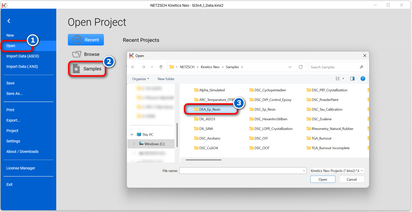
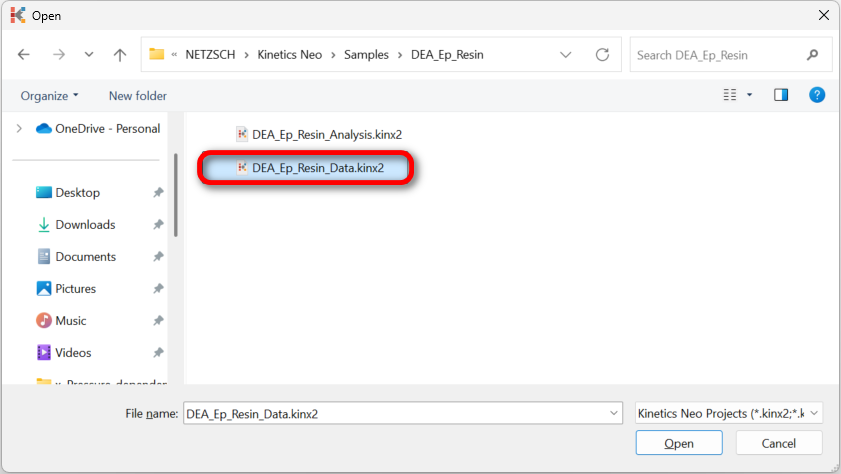
3. Open Kinetics Neo project file DEA_Ep_Resin_Data.kinx2 .

Check the Loaded Measurement Data

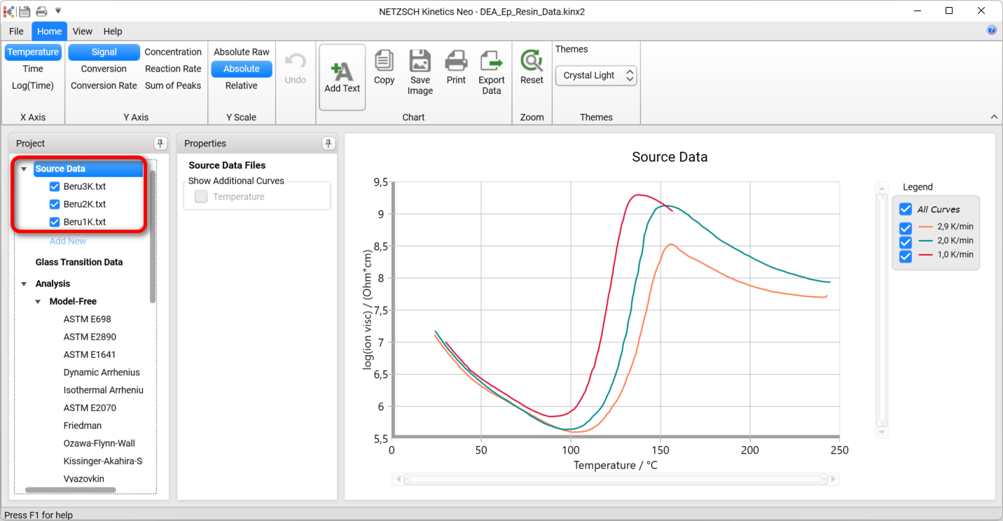
4. Check if the DEA measurement data are loaded.

The Kinetics Neo sample project DEA_Ep_Resin_Data.kinx2 already contains imported sample DEA data files of Curing of Epoxy Resin:

• Beru3K.TXT – heating rate 3K/min
• Beru2K.TXT – heating rate 2K/min
• Beru1K.TXT – heating rate 1K/min

If the project file is successfully loaded then these file names will be seen in Source Data section on the right side. The data curves will be shown on the main chart.

Baseline correction

Dielectric data during the temperature initialized cure of a resin is depending on the progressive cross-linking and the increasing temperature that yield to effects in the opposite direction. Thus, a baseline for the temperature effect has to be constructed.

Kinetics Neo delivers baseline models for different curing conditions. In the case shown here, a dynamic curing at a constant heating rate was performed. The molecular mobility of the resin due to temperature is influenced before as well as after the curing progress. The temperature effect on molecular motion in dielectric data can be described using exponential functions based on Arrhenius fundamentals and is done by using the button Tangential (DEA dynamic). This creates an exponential function to the point where the cursor is located to.

5. Select the first data file Beru3K.txt, select temperature range between 53 °C and 180 °C and select Tangential (DEA Dynamic) baseline.

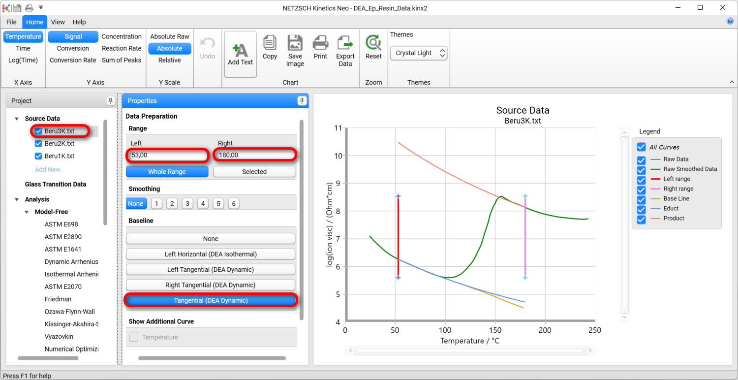
Here calculated blue curve shows temperature dependence of ion viscosity for uncured state. Calculated orange curve shows temperature dependence of ion viscosity for fully cured state. Brown curve presents the common baseline, which changes its slope from uncured to cured state. This common baseline will be subtracted from the total measurement in order to have only curing effect.

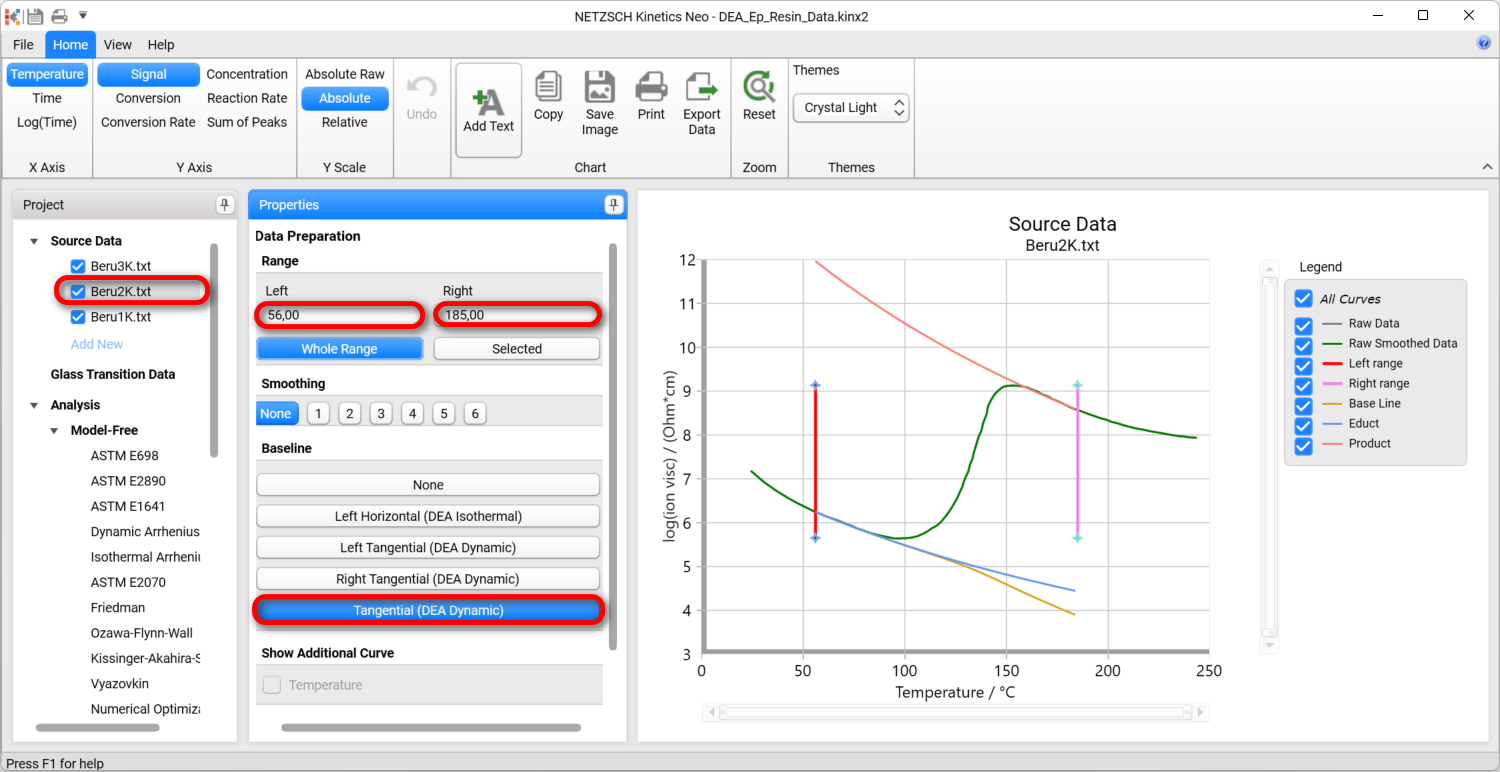
6. Select the second data file Beru2K.txt, select temperature range between 56 °C and 185 °C and select Tangential (DEA Dynamic) baseline.

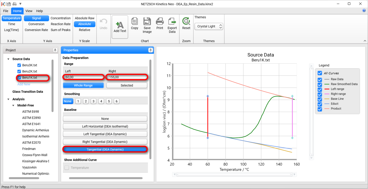
7. Select the third data file Beru1K.txt, select temperature range between 60 °C and 155 °C and select Tangential (DEA Dynamic) baseline.

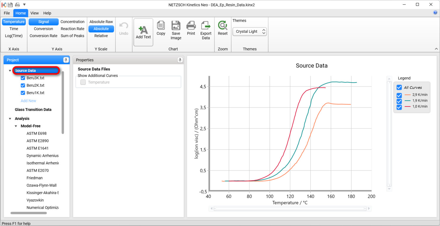
8. Click on Source Data in the left Project panel. Now all measured curves contain only effect of curing.

Create a Single Step Kinetic Model for Curing Effect

9. Add new model: In Analysis left panel under Model Based item click on Add New.
 

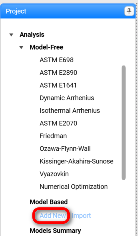
A new Model Based kinetic model will be created with default parameters:

• one step: A → B
• Reaction type: F1, 1^st order reaction.

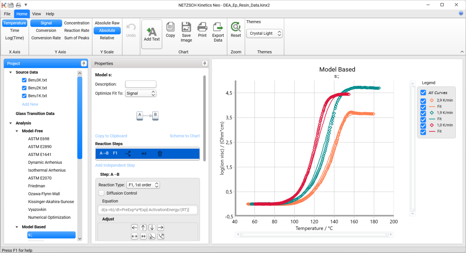
10. Change reaction type for A → B kinetic step

It is known that curing reactions are usually autocatalytical reactions. In this case it is recommended to select reaction with autocatalysis with unknown reaction order n and unknown order of autocatalysis. Using model optimization the software will determine the correct reaction order by itself.

Select step A → B, select reaction type Cn.

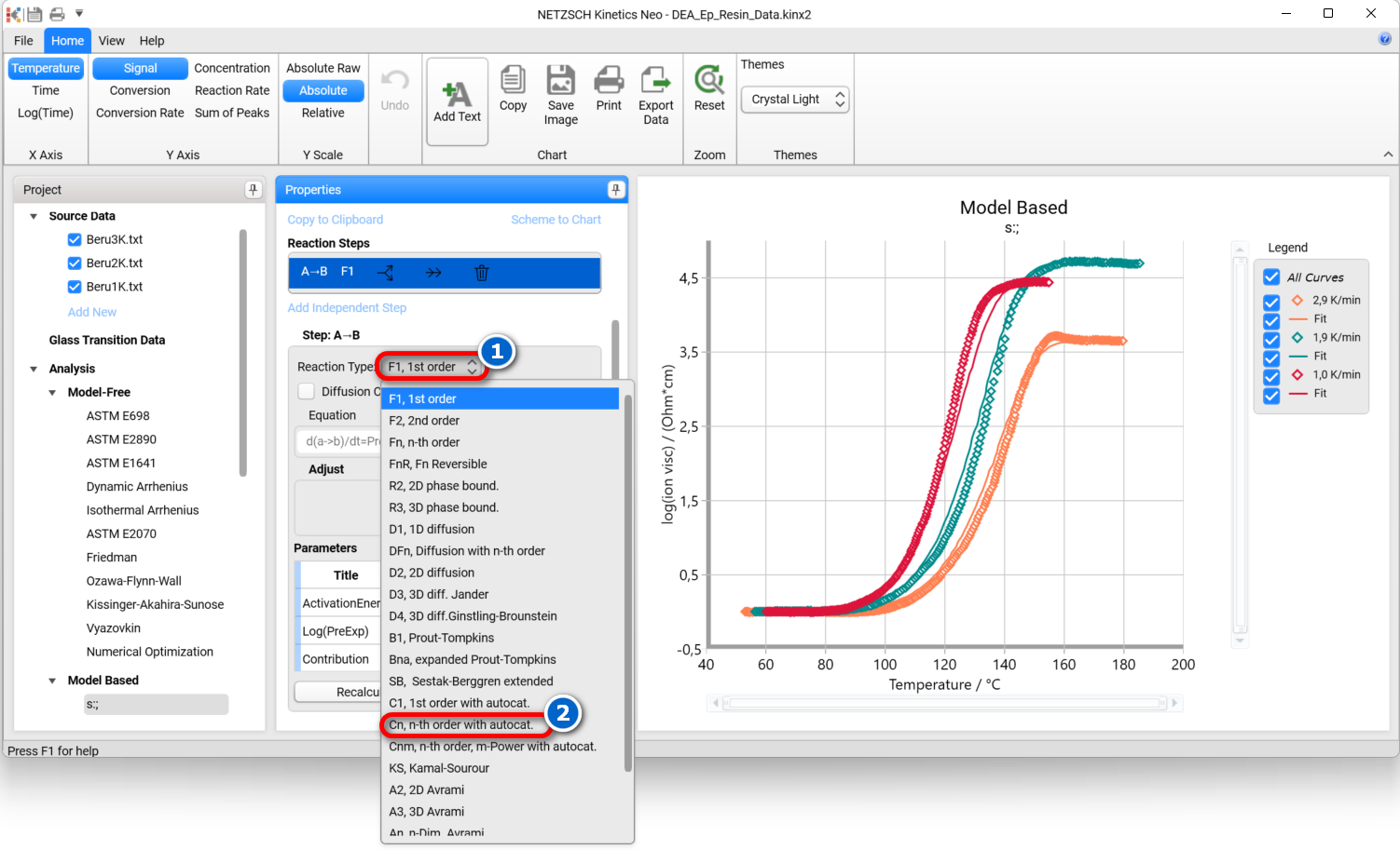
Result after changing of reaction type to Cn:

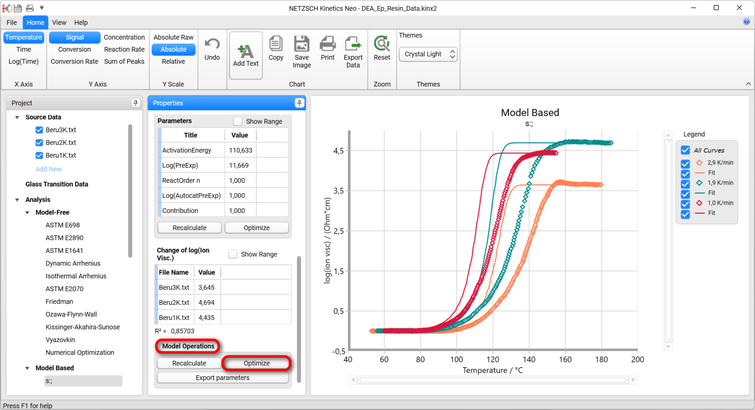
11. Optimize one-step model.

Select Optimize in Model Operation block at the lower part of Properties panel.

The model step will be optimized. This may take some seconds...

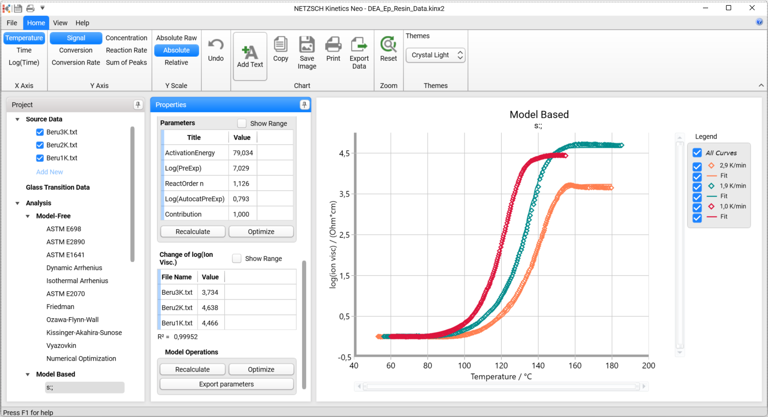
One-step kinetic model is ready:

Apply model free method to DEA data

12. The model-free methods could be found in the left panel Project in the section Analysis / Model-Free.

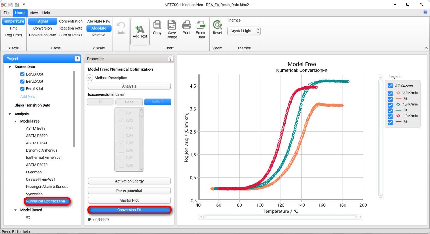
Apply model-free method: in Analysis left panel under Model-Free item click on Numerical Optimization. Then click on Conversion Fit in the second panel Properties. 

 The model-free Numerical method is applied for the increasing of ion viscosity during curing. Here the baseline is removed and not taken into account. 

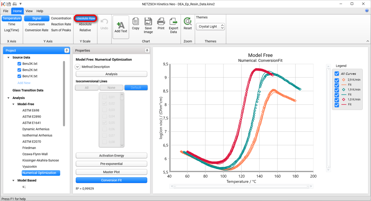
13. Switch to Absolute Raw for Y Scale in the horizontal Toolbar.

Now the original measured data for ion viscosity and model-free fit for them is presented.

For the further prediction and optimization one of kinetic results (model-based or model-free) can be selected.