How To: Analyze Isothermal Data Of OIT (Oxidation Induction Time) And Create OIT Predictions
Introduction
For each isothermal measurement the time-to-event value is important: this is the time point at which the material has defined changes.
Typical examples are:
- OIT (Oxidation Induction Time) –the time of oxidation start for material stored in air
- rupture of the sample under mechanical stress like in isothermal DMA tests
- initial part of thermal degradation of packages with mass loss about 5-10%.
From each measurement the pair of values are taken for analysis:
- temperature
- time-to-event.
Analysis shows graphic Log of time-to-event vs inverse temperature as the straight line. Activation energy and pre-exponential are found from the slope and intersect of this line.
Advantage of this method:
- No entire measurement required, just the time-to-event.
Disadvantages of this method:
- only one-step reactions, for complex reactions the points are not on the straight line
- only for the set of several isothermal measurements
- only one point is evaluated, all other information is lost.
Method Source: ASTM 2070, Method D.
Create Kinetics Neo Project for Isothermal OIT Analysis
Create new project of DSC type. For other events like TGA or DMA another project type can be created.
1. Start the Kinetics Neo software. Click on the blue "File" tab to open the application menu.
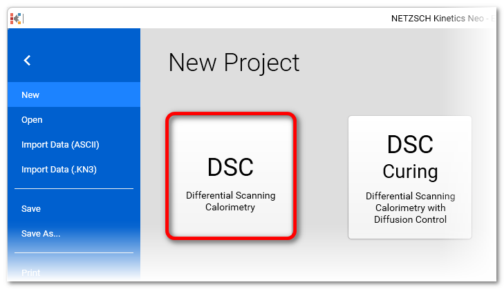
2. In blue Application Menu select New and click on "DSC".
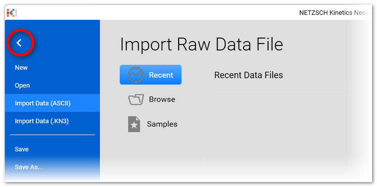
3. IMPORTANT - Return back in order to input data manually. Click on "Back" button on the top left side.
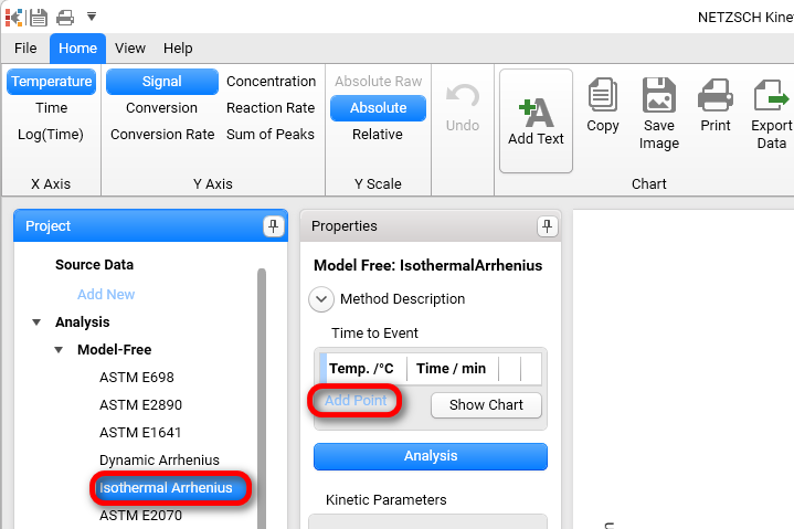
4. Add the first data point: isothermal temperature and corresponding OIT time.
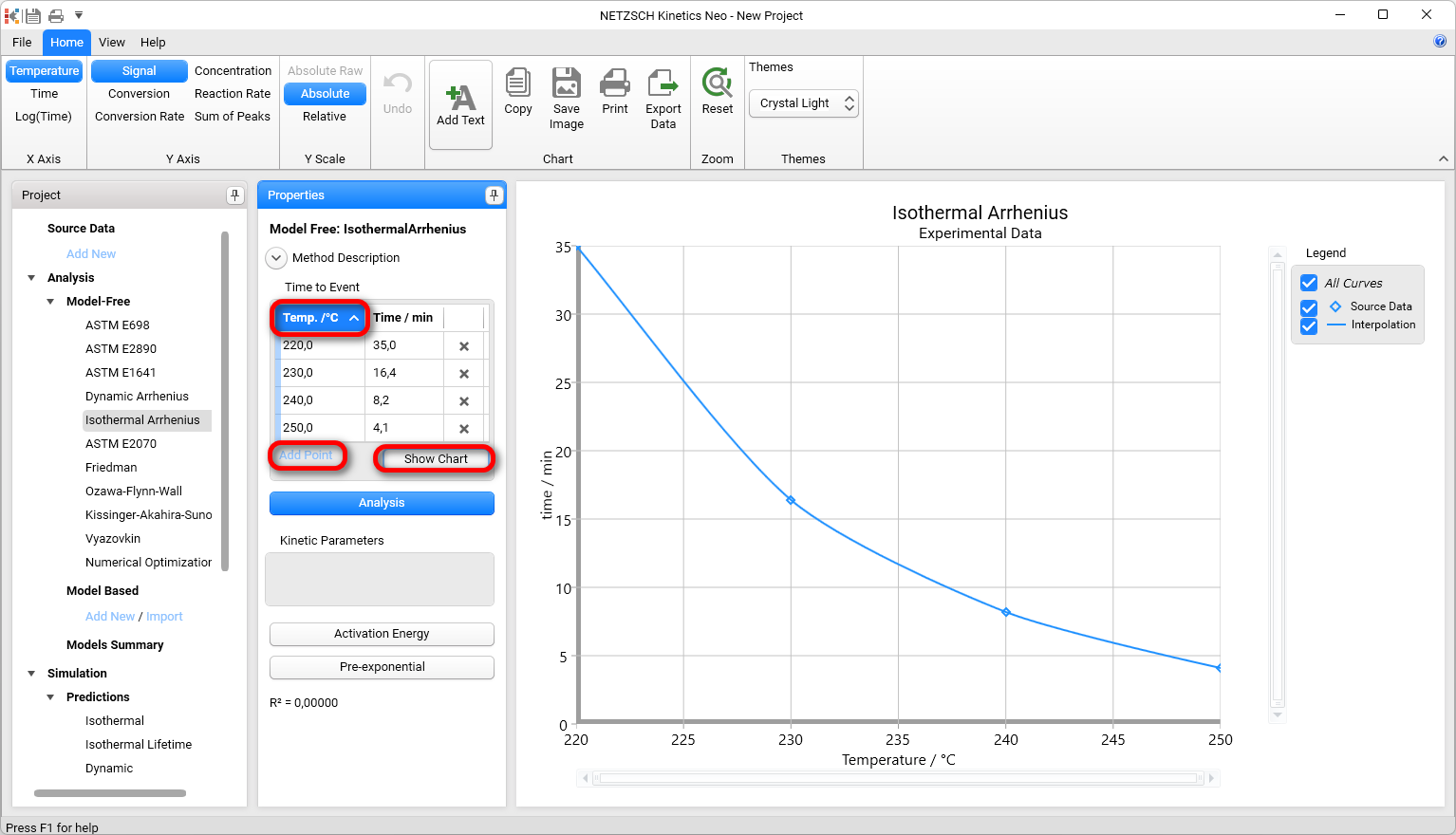
In the left tree select Project --> Analysis --> Model-Free --> Isothermal Arrhenius and press Add point in Properties panel:
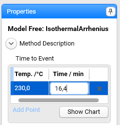
5. Type temperature 230°C and time 16.4 min .
6. Using Add point please add three additional the time-to event values for temperatures:
- 220°C - 35 min
- 240°C - 8.2 min
- 250°C - 4.1 min
Click on Temp column header to soft the table by increasing of temperature values.
Click Show Chart:
7. Click on Analysis button to calculate Arrhenius plot and kinetics parameters:
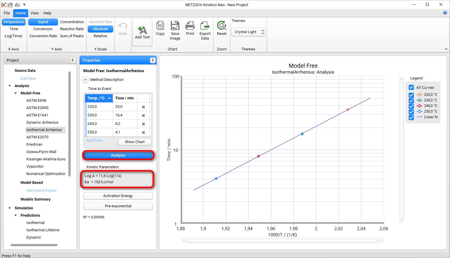
Here the activation energy is calculated from the slope of Arrhenius graph, and Pre-exponential factor is calculated under the assumption of the first-order reaction and 5% conversion at the OIT point.
8. Now these kinetic parameters belong to Isothermal Arrhenius model and can be used for any predictions.
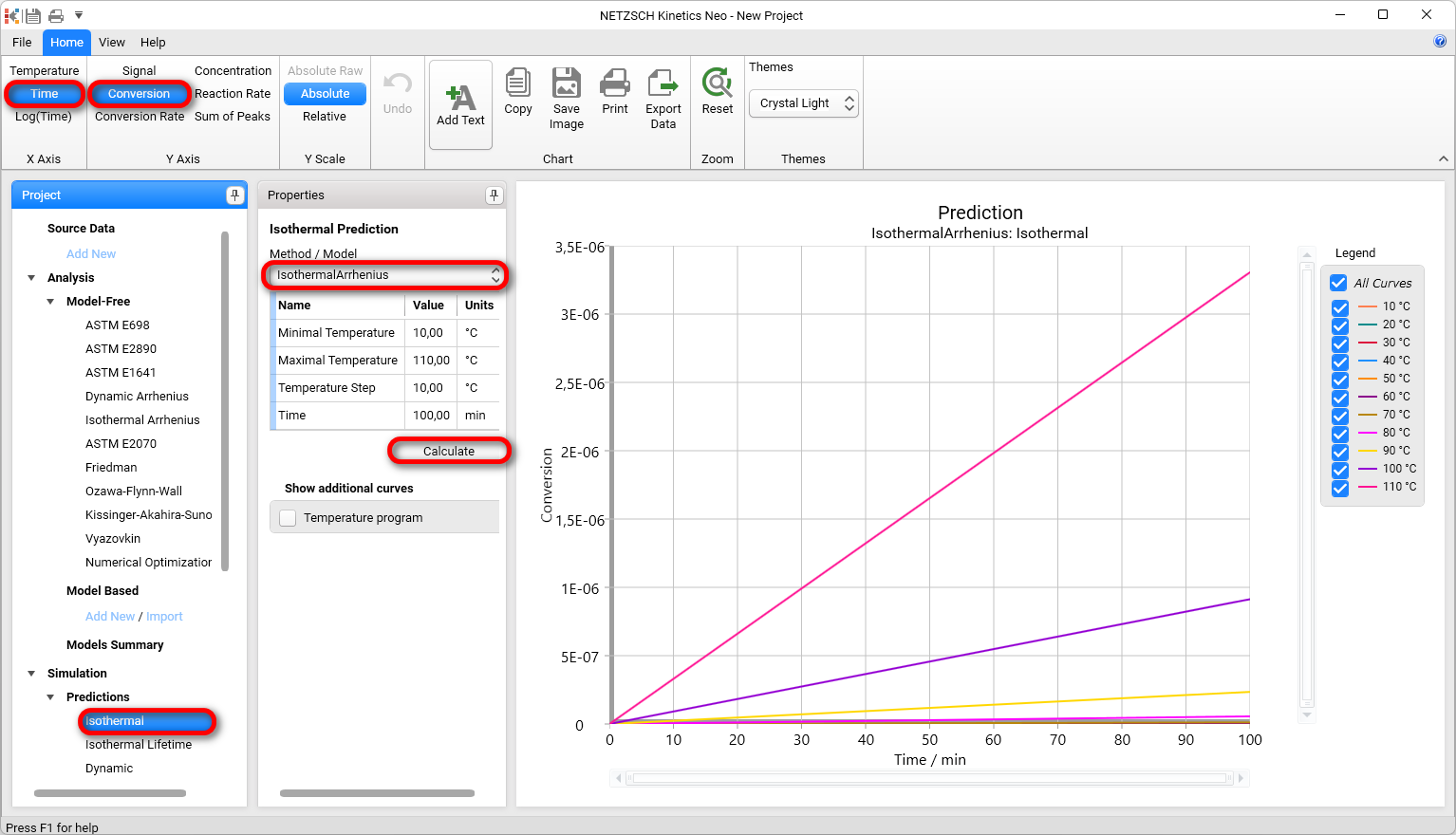
Select Isothermal in Simulation - Predictions section of the Project panel. Then select Time as X Axis and Conversion as Y Axis.
Check that Isothermal Arrhenius is selected in Method / Model list and click on Calculate:
Change the parameters of Isothermal prediction as it shown below:
- Mininal Temperature: 220 °C
- Maximal Temperature: 250 °C
- Temperature Step: 10 °C
- Time: 50 min.
Click on Calculate.
Drag the top edge of the vertical chart scroll bar down to set the maximum Y value to approximately 0.05.
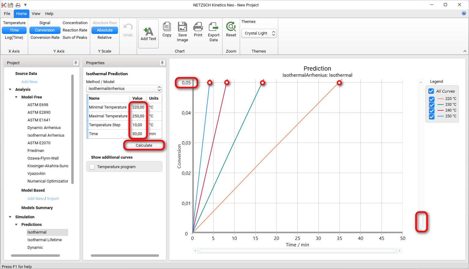
Here the Conversion curves type is selected and then zoomed from 0 to 5%. We see, that isothermal predictions for 220°C, 230°C, 240°C and 250°C by Isothermal Arrhenius method show 5% of conversion from 4.8 to 35 minutes .
Isothermal Lifetime Prediction: Prediction of OIT (Oxidation Induction Time)
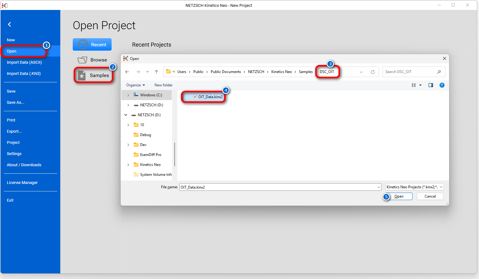
1. We will use sample Kinetics Neo project OIT_Data.kinx2.
Click on File on the main ribbon and then on Open. Select Samples on the right panel.
Go to folder DSC_OIT and open file OIT_Data.kinx2.
In the left Project panel select Isothermal Arrhenius in Model Free section to show experimental OIT data.
These are four experiments at temperatures 230°C, 230°C, 240°C and 250°C with measured oxidation induction time (OIT) for each of these temperatures. Click on Analysis in order to see Arrhenius plot for these data.
This model Isothermal Arrhenius can be used for the isothermal Lifetimepredictions in order to predict time-to-event (OIT) for other temperatures.
In the left tree select Simulation → Prediction → Isothermal Lifetime. Then in drop down model menu select Isothermal Arrhenius , set
- Minimal Temperature to 220°C,
- Maximal Temperature to 250°C,
press Calculate.
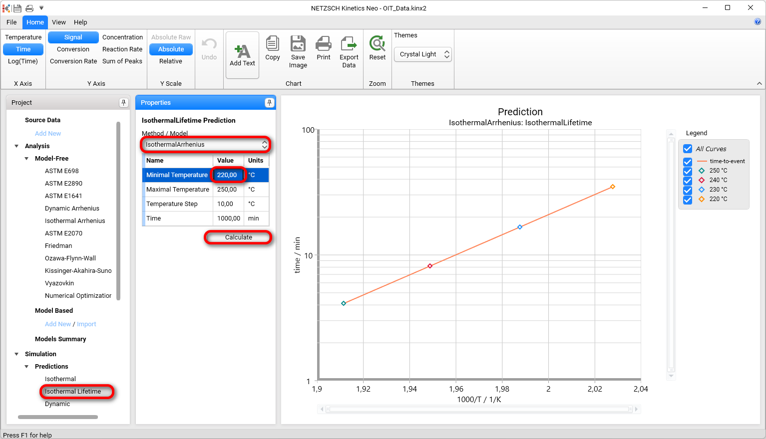
Now we see the same Arrhenius plot like in Step 1. But here each point is simulated.
If we want to find OIT time at 200°C, then we should set Minimal Temperature = 200°C, and the time, which is long enough to reach OIT at lower temperature.
Click on Calculate:
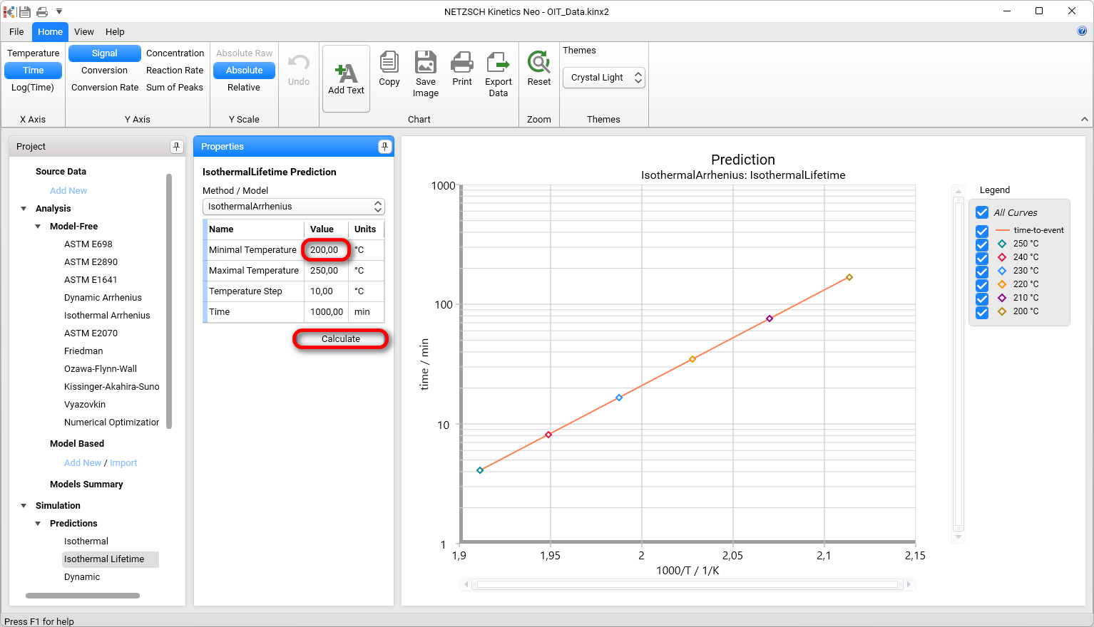
The last point shows OIT time for isothermal measurement 200°C. This means that OIT for 200°C is almost 3 hours.
In order to see the predicted time values, please click on Export Data button on the toolbar.