How To: Create a Simple Single Step Kinetic Model for ARC Data (Constant Power Mode)
Thermal decomposition of the mixture DTBP (di-tert-butyl peroxide) in toluene
Contents
Short Description of ARC Constant Power Measurement
Check the Loaded Measurement Data
After - Import Sample Data Preparation
First Source File "5percent_DTBP_250mW.txt"
Second Source File "10percent_DTBP_250mW.txt"
Third Source File "15percent_DTBP_250mW.txt"
Check the Loaded Measurement Data After Selecting Data Range and Baseline
Introduction
In this "How To", a simple single-step kinetic model for the ARC temperature curves will be created. The measurements performed with different concentrations of DTBP in toluene will be used. The keypoint of this document is how to prepare the data measured by accelerating calorimeter and how to select and apply the correct baseline.
Sample Data:
Data Type: Accelerating Rate Calorimetry (ARC), Constant Heat mode.
Measurement Data Files:
- 5percent_DTBP_250mW.txt
- 10percent_DTBP_250mW.txt
- 15percent_DTBP_250mW.txt
Kinetics Neo project files:
- ARC_Temperature_DTBP_Data.kinx - contains a set of measurement data only, it is a start point for this "How To:";
- ARC_Temperature_DTBP_Analysis.kinx - contains additionally source data correction and kinetic model created in this "How To:".
Short Description of ARC Constant Power Measurement
This method measures the temperature increase of the exothermal reaction by means of:
- ARC (Accelereting Scanning Calorimetry),
- APTAC (Automatic Pressure Tracking Adiabatic Calorimeter) or
- MMC (Multiple Mode Calorimeter).
In the Constant Power mode the heaters continuously inputs the constant amount of heat energy throughout the measurement. There is no variation in the power input regardless of the sample self-heating.
In this mode the temperature has the linear increase for the ranges without reaction and temperature step during the exothermal reaction:
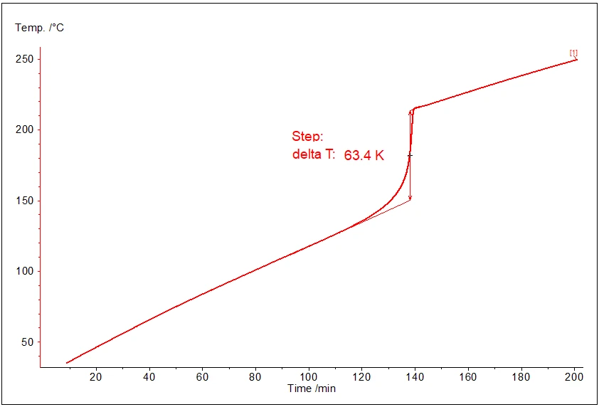
The picture shows typical behavior of temperature at constant power measurement:
- linear increase before the reaction,
- step increase during the reaction (after 120 minutes sample begins to evolve heat),
- linear increase again after the reaction.
Load the Sample Data Project
Start the Kinetics Neo software.
1. On the top left click on the blue "File" tab to open the application menu.
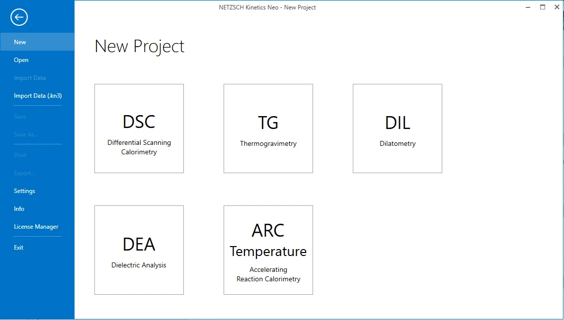
2. Open the sample data ARC Temperature project.
Click on "Open" in the menu on the left side, then select "Samples". The Kinetics Neo samples directory will be opened in Windows Explorer. Select the directory “ARC_Temperature_DTBP”.
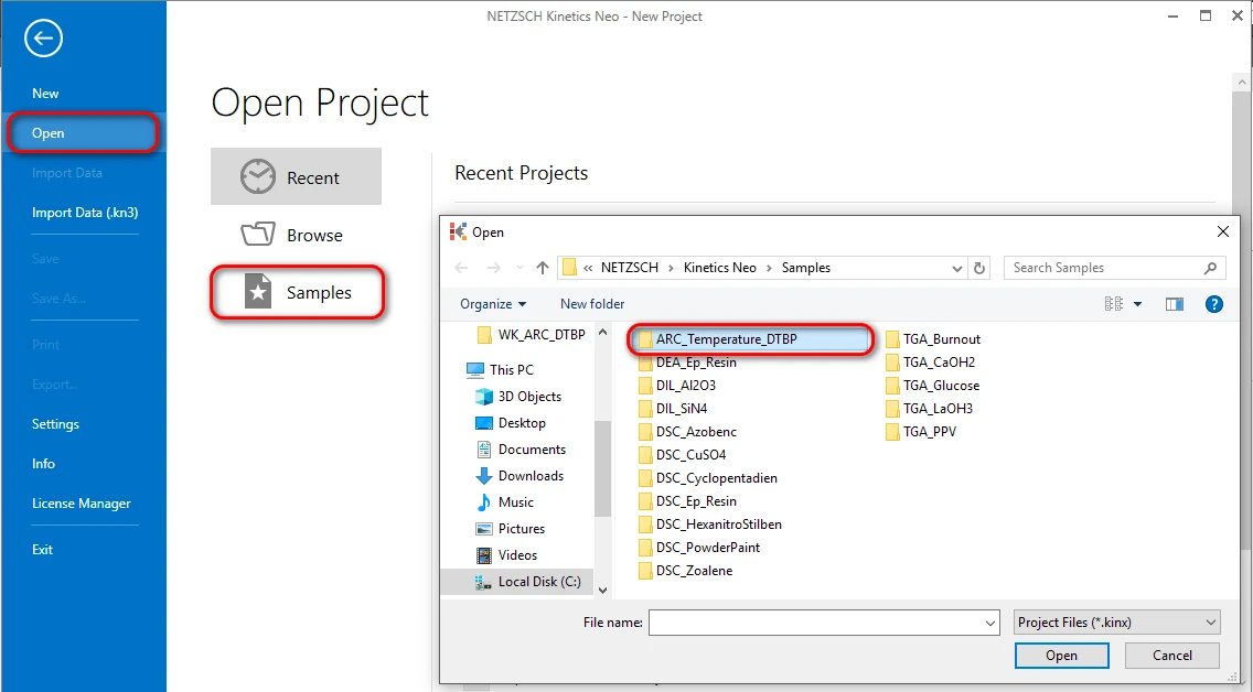
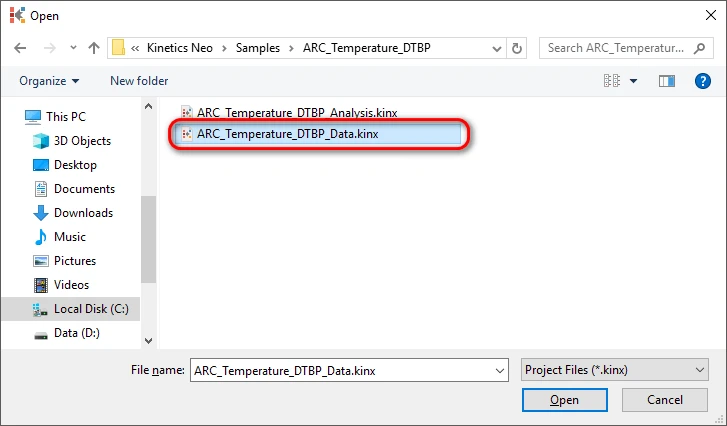
3. Open the Kinetics Neo project file “ARC_Temperature_DTBP_Data.kinx”.
Check the Loaded Measurement Data
4. Check whether the ARC Temperature (Constant Power mode) measurement data are loaded.
The Kinetics Neo sample project "ARC_Temperature_DTBP_Data.kinx" already contains sample ARC Temperature measurement data files for Constant Power measurement:
- 5percent_DTBP_250mW.txt - 5% solution of DTBP in toluene, constant power 250 mW,
- 10percent_DTBP_250mW.txt - 10% solution of DTBP in toluene, constant power 250 mW,
- 15percent_DTBP_250mW.txt - 15% solution of DTBP in toluene, constant power 250 mW.
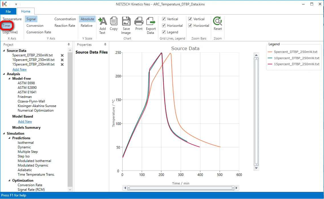
If the project file is successfully loaded then these file names will be seen in the "Source Data" section on the left side. The data curves will be shown on the main chart.
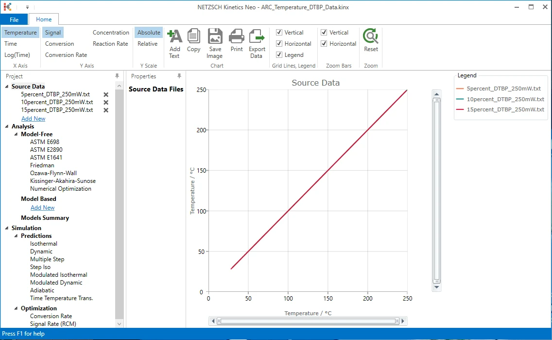
5. Switch to a time X-axis
On the top ribbon in the left side click on "Time" to select time X-axis. Now all three data curves are visible.
After - Import Sample Data Preparation
By clicking on one of the sample data files it would be possible to narrow the data range by selecting a left and a right range position. In addition smoothing of the data can be done if necessary.
Baseline could also be applied.
First Source File "5percent_DTBP_250mW.txt"
Select the Source File
6. On the left Project panel under Source Data click on the "5percent_DTBP_250mW.txt" item. The Data Preparation properties panel and the chart of selected source data file will be shown:
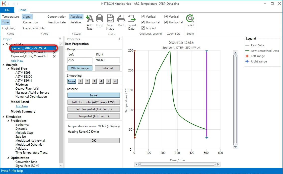
Select a Data Range
The exothermal reaction is detected here as the step on the temperature curve at approximately 150 minute.
We need to adjust the data range so that it will contain the vertical temperature step and both linear parts of the curve before and after the step.
Left Data Range
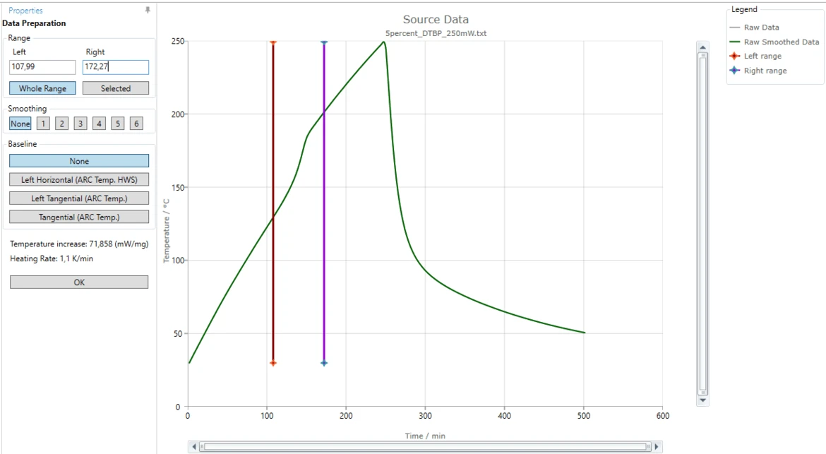
Red vertical line represents the left range of analyzed source data.
7. Move the mouse pointer to this vertical red line. The mouse cursor will change his image to <->. Now left data range can be adjusted.
8. Press and hold the left mouse button over the red vertical line and in the same time move the cursor to the right ("drag" the line). The left data range line will follow the mouse cursor.
9. Release the left mouse button ("drop") when the red line is approximately at 108 minute.
Alternatively, in the "Left" text box in "Range" area of "Data Preparation" panel you can type "107,99". The nearest data point to the right will be selected as left data range border.
Right Data Range
10. Repeat the same procedure with the violet vertical line which represents the right data range.
Move this right range line to approximately 172 minute.
Alternatively, in the "Right" text box in "Range" area of "Data Preparation" panel you can type "172,27". The nearest data point to the left will selected as right data range border.
Select a Baseline
For exothermal reactions measured by acceleration calorimeter the background heating can be applied. Therefore the baseline should be selected to remove this background heating. The options are:
- None;
- Left Horizontal (ARC Temp HWS);
- Left tangential (ARC Temp);
- Tangential (ARC Temp).
11. Select a correct baseline: for this "How To" please select the baseline type Tangential (ARC Temp.), because the slope of the measured curves before and after the reaction are different.
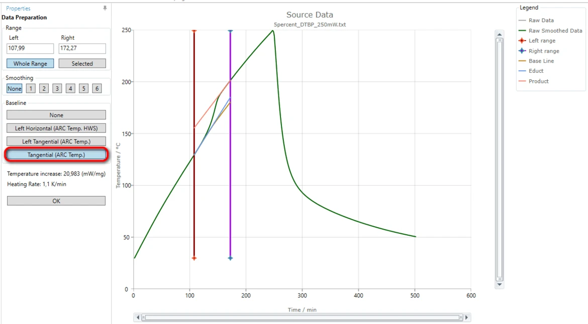
The blue tangent is created for the left linear part of the measured curve before the step. The orange tangent is created for the right linear part after the step.
The brown curve is the common baseline having left slope equal to the left tangent and right slope equal to the right tangent.
This common calculated baseline will be removed from the measured curve in order to have adiabatic temperature increase only.
By moving the left or right range border lines (red or violet vertical lines) the range selection can be improved so, that the both tangents have good agreement with the corresponding linear parts of the measured curve.
Save Adjustments Made to the Source File
12. Save your changes: after range and baseline selection press OK button in Data Preparation panel.
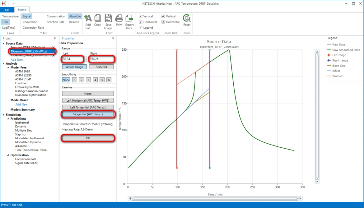
Second Source File "10percent_DTBP_250mW.txt"
13. Select the second measurement file: on the left Project panel under Source Data click on the "10percent_DTBP_250mW.txt" item. The Data Preparation properties panel and the chart of selected source data file will be shown.
14. Adjust the data range to approximately:
- Left: 91,69 minute,
- Right: 166.70 minute.
15. Select the same baseline "Tangential (Arc.Temp)" as for previous data file.
Third Source File "15percent_DTBP_250mW.txt"
16. Repeat the same steps as done before for the second data file "15percent_DTBP_250mW.txt".
Check the Loaded Measurement Data After Selecting Data Range and Baseline
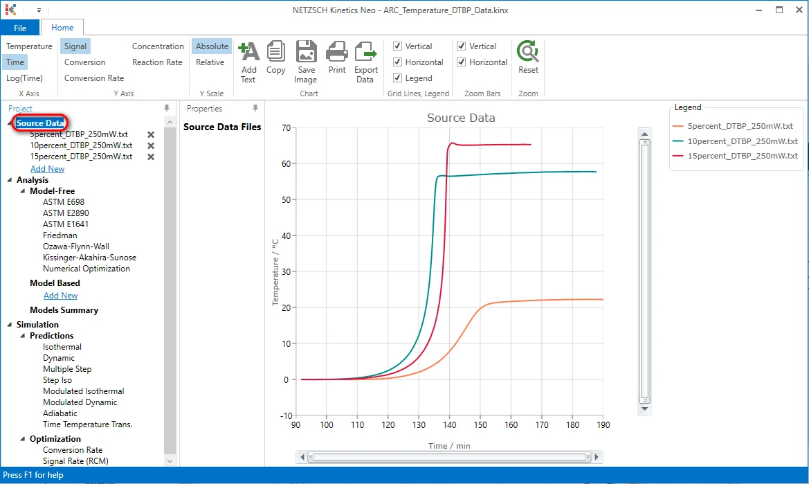
Create a One-Step Kinetic Model
After loading the source data, adjusting their range and applying the baseline we can start with kinetic modelling.
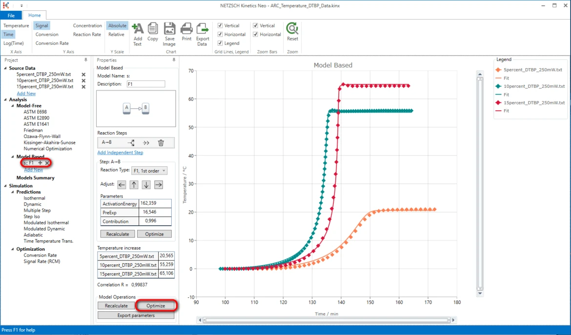
17. Add new kinetic model: on the left Project panel in Analysis tree under Model Based click on Add New to create the kinetic model.
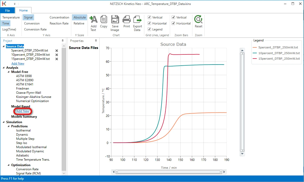
A new “Model Based” kinetic model will be created.
This new model has the following default parameters:
- One step: A->B.
- Reaction Type: F1, 1st order.

The first model can be a reaction of 1st order.
During creating of a new kinetic model, the software sets the initial values for all parameters.
IMPORTANT: It is always recommended to optimize these initial step parameters first.
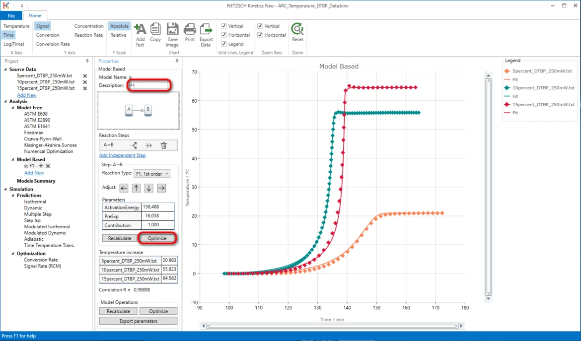
18. Optimize step parameters after creating a new kinetic model: in Model Based properties panel in Step: A->B area click on Optimize. It will take some seconds to optimize the model.
It is always recommended to add some comment or description to the model.
19. Write "F1" In the field Description.
20. Optimize the whole kinetic model: in the section Model Operations click on Optimize.
Results
21. Now the simulated data are in good agreement with the experiment.
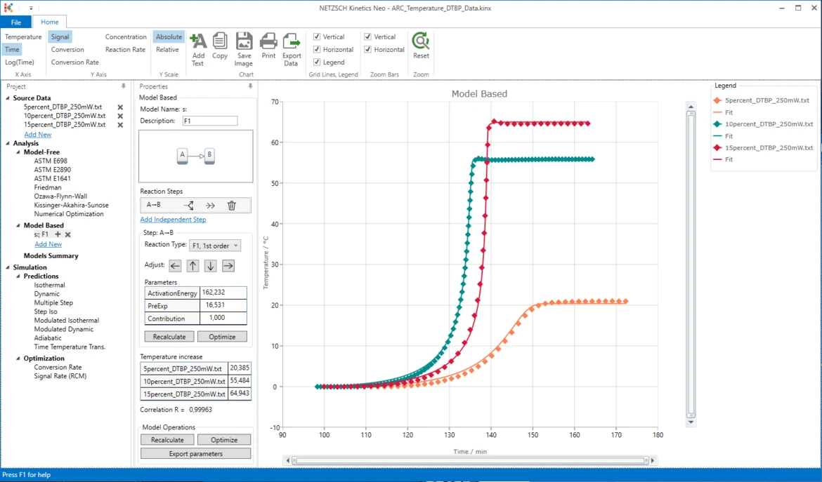
Conclusion
The decomposition of DTBP can be described as a the one-step reaction of the first order without autocatalysis.